ANOVA In Excel

ANOVA in Excel is a built-in statistical test used to analyze the variances. For example, we usually compare the available alternatives when buying a new item, which eventually helps us choose the best from all the available options. Using the ANOVA test in Excel can help us test the different data sets against each other to identify the best from the lot.

ANOVA tests the null hypothesis that all group means are equal and is available in Excel under the Data Analysis Toolpak. There are different types of ANOVA: Single Factor (one independent variable) and Two-Factor (two variables).

Assume you conducted a survey on three different flavors of ice creams, and you have collated opinions from users. Now, you need to identify which flavor is best among the views. Here, we have three different flavors of ice creams. These are called alternatives, so we can locate the best from the lot by running the ANOVA test in Excel.

ANOVA is not a function in Excel. However, if you have already tried to search for ANOVA, you may have failed because it is part of Excel's "Data Analysis" tool.

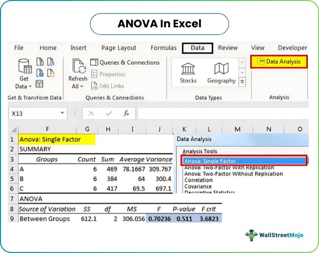
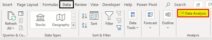
Data Analysis is available under the "DATA" tab in Excel.

If you cannot view this in your Excel, follow the below steps to enable "Data Analysis" in your Excel workbook.

Enabling the Data Analysis ToolPak in Excel

1. Click on "FILE" and "Options".

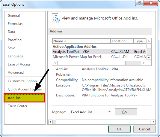
2. Click on "Add-Ins."

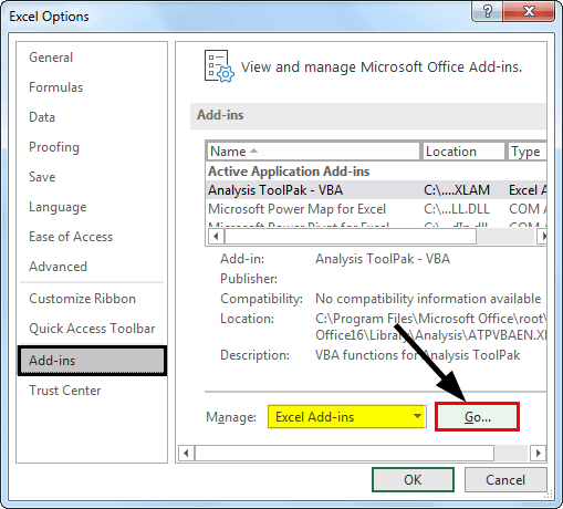
3. Under "Add-Ins," select "Excel Add-Ins" from the "Manage" options and click on "Ok."

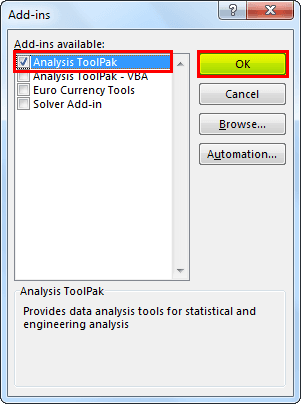
4. Now, from the below window, select "Analysis Toolpak" and click on "OK" to enable it.

You should see “Data Analysis” under the “DATA” tab.

Conducting an ANOVA test in Excel is a technical approach that needs proper training. If you wish to acquire some basic understanding of how to conduct such tests before you proceed to the next section, you can surely have a look at this Data Analysis In Excel course.

One-Way ANOVA in Excel Example

The following is an example of how to do an ANOVA test in Excel.

For this example, consider the below data set of three students’ marks in 6 subjects.

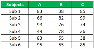
Above are students' A, B, and C scores in 6 subjects. Now, we need to identify whether the scores of three students are significant or not.

• Step 1: Click on "Data Analysis " under the Data tab."

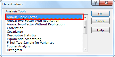
• Step 2: In the “Data Analysis” window, select the first option, “Anova: Single Factor.”

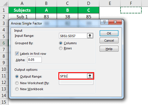
• Step 3: In the next window for “Input Range,” select student scores.

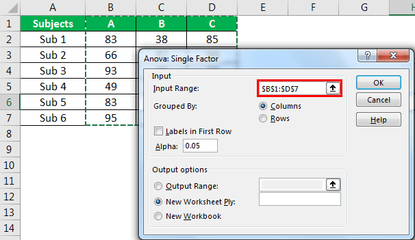
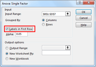
• Step 4: Since we have selected the data with headers, check the box “Labels in First Row.”

• Step 5: Now select the “Output Range” as one of the cells in the same worksheet.

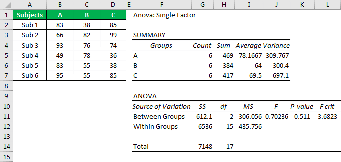
• Step 6: Click on “OK” to complete the calculation. Now we will have a detailed “Anova: Single Factor” analysis.

Before we interpret the results of ANOVA, let us look at the hypothesis of ANOVA. Then, to compare the Excel ANOVA test results, we can frame two hypotheses – the "Null hypothesis" and "Alternative hypothesis."

The null hypothesis is "there is no difference between scores of three students."

The alternative hypothesis is that "at least one of the means is different."

• If "F value > F critical value," we can reject the null hypothesis.
• If "F value < F critical value," we cannot reject the null hypothesis.
• If "p-value < alpha value," we can reject the null hypothesis.
• If "p-value > alpha value," we cannot reject the null hypothesis.

Note: alpha value is the significance level.

You may not go back and look at the result of ANOVA.

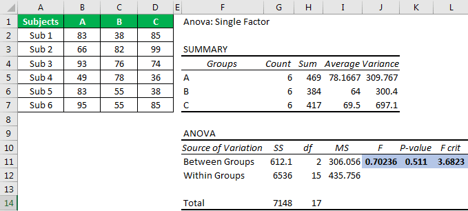
First, look at the "p-value," which is 0.511. Unfortunately, it is greater than the alpha or significance value (0.05), so we cannot reject the null hypothesis.

Next, the F value of 0.70 is less than the F critical value of 3.68, so we cannot reject the null hypothesis.

Next, the F value of 0.70 is less than the F critical value of 3.68, so we cannot reject the null hypothesis.

As we explore the complexities of this topic, it becomes clear how foundational knowledge can lead to practical applications. Those interested in enhancing their skills further might find this basic power pivot course helpful for gaining deeper insights.

Two-Way ANOVA in Excel

If there are now two factors, we need a two-way ANOVA instead of a one-way one.

For this, click on the Data Analysis icon. 

We get a dialog box with two different options for a two-way ANOVA.

You can either choose from:

• ANOVA: Two-Factor With Replication: Used for multiple observations, or replications
• ANOVA: Two-Factor Without Replication: Used when we have only one observation.

You can always ho-ahead and consider taking our Advanced Excel course for increasing your knowledge so that it is easy to handle tough topics like ANOVA.

• Equal sample sizes are not required, but they improve the reliability of the test results.
• Always frame the null hypothesis and the alternative hypothesis.
  • If the F value > F critical value," then we can reject the null hypothesis
• "If F value < F critical value," we cannot reject the null hypothesis.
• Only numeric data should be included, else we may get errors.