Pivot Chart In Excel

PivotChart in Excel is an in-built program tool that helps you summarize selected rows and columns of data in a spreadsheet. The visual representation of a PivotTable or any tabular data helps summarize and analyze the datasets, patterns, and trends. Simply put, a pivot chart in Excel is an interactive Excel chart that outlines large amounts of data.

For example, one can create a pivot chart to show the total sales by region and product category. It gets updated automatically when you filter or rearrange fields in the pivot table.

Let us learn how to create a PivotChart in Excel with the help of an example. Here, we do the sales data analysis.

Below mentioned data contains a compilation of sales information by date, salesperson, and region. Here, we need to summarize sales data for each representative regionally in the chart.

Step 1: We must first select the data range to create a PivotChart in Excel.

Step 2: Then, click the "Insert" tab within the ribbon.

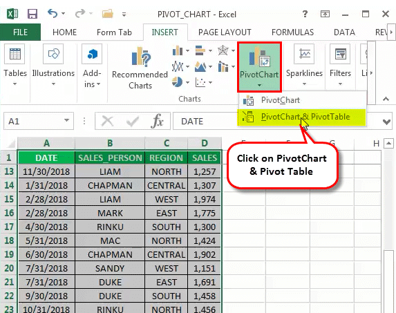
Step 3: Then, select the "PivotChart" dropdown button within the "Charts" group. 

So, for example, if we want only to create a PivotChart, choose "PivotChart" from the dropdown or if we are going to make both a PivotChart and PivotTable, then select "PivotChart & PivotTable" from the dropdown.

Step 4: Here, we have selected and created both a PivotChart and PivotTable. Then, make PivotChart, a dialog box appears, similar to the "Create PivotTable" dialog box. 

It will ask for the options: Table/Range or Use an external data source. By default, it selects "Table/Range," which will ask where to place a PivotTable chart. Here, we always need to choose a new worksheet.

Step 5: Clicking "OK" will insert PivotChart and PivotTable into a new worksheet.

Step 6: “PivotChart Fields” task pane appears on the left, containing various fields: Filters, Axis (Categories), Legend (Series), and Values. Next, in the PivotTable Fields pane, select the "Column" fields applicable to the Pivot Table. 

Then, we can drag and drop, i.e., "Sales_person" to the "Rows" section, "Region" to the "Columns" section, and "Sales" to the "Values" section.

Then, the chart looks as given below.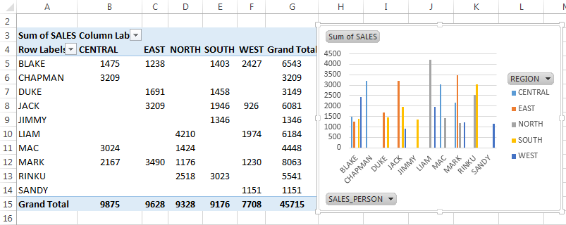

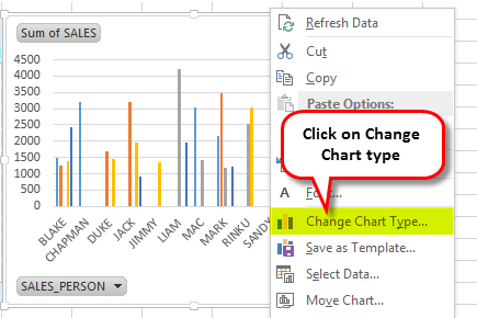
Step 7: We can name this sheet "SALES_BY_REGION" by clicking on the PivotTable. Then, we can change the chart type in the "Change Chart Type" option based on choice under the "Insert" tab. Select "PivotChart, and" the "Insert Chart" popup window appears. Under that, select the "Bar" and "Clustered" bar chart. Then, right-click on the PivotChart, and choose "Change Chart Type."

Step 8: Under "Change Chart Type," select "Column." Then, select the "Clustered Column" Chart.

Step 9: Now, we can summarize the data with the help of interactive controls present across the chart. For example, when we click on the "Region" filter control, a search box appears with the list of all the regions, where we can check or uncheck boxes based on the choice.

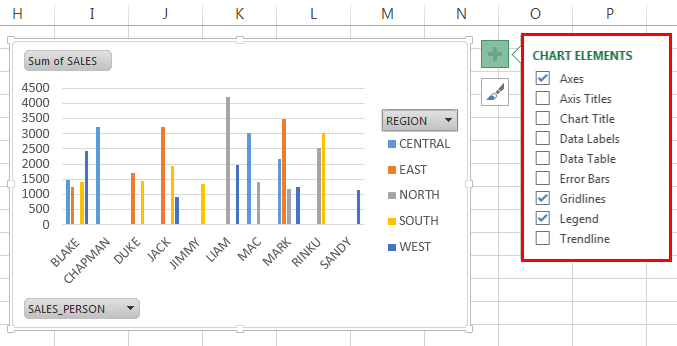
Step 10: On the corner of the chart, we have an option to format chart elements based on the choice.

Step 11: We have an option to customize the PivotTable "Values." By default, Excel uses the SUM function to calculate the values available in the table. Suppose we select only region values in the chart; it will display each region's total SUM sales.

Step 12: We have an option to change the Excel chart style by clicking the "Style" icon on the corner of the chart.

This chart will update when we change data sets in a PivotTable. The following steps can optimize this option: right-click and select the "PivotChart Options".

In the above chart options, go to the "Data" tab and click on the checkbox "Refresh data when opening a file." So that refresh data gets activated.

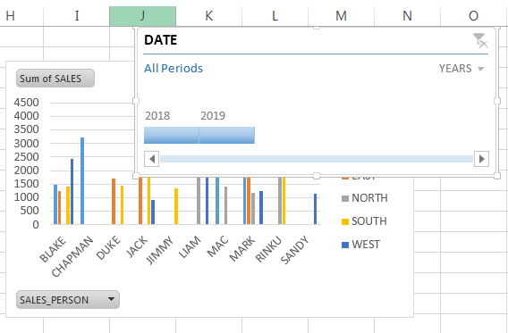
In an Excel PivotChart, we can insert a timeline to filter dates (monthly, quarterly, or yearly) in a chart to summarize sales data (This step applies when the dataset contains only date values).

We can also use a "Slicer" with a PivotChart to filter region-wise data or other field data of the choice to summarize sales data.