Regression Analysis In Excel

Regression Analysis in Excel defines relationships between two or more variables in a data set. Regression analysis helps examine the relationship between a dependent variable and one or more independent variables. It is used to predict trends and understand data patterns in Excel. In statistics, regression is done with the help of some complex formulas. However, in Excel, we have suitable tools to perform Regression Analysis.

For example, to calculate the Regression Analysis in Excel for an input range with X and Y valuesrange, perform the following steps. S

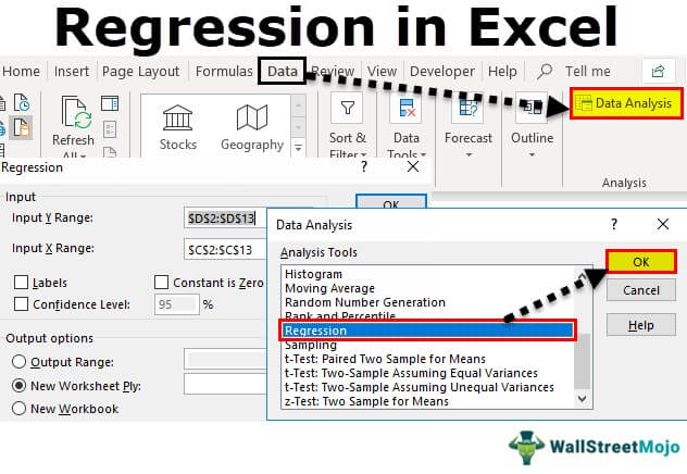
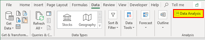
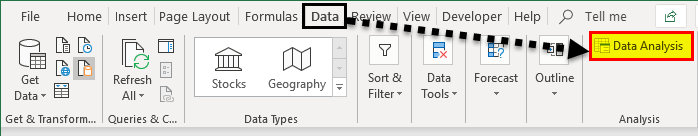
• Select the "Data" tab
•  Go to the "Analysis" group
• Click the “Data Analysis” option
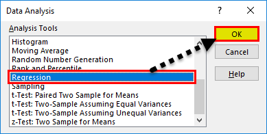
• When the "Data Analysis" window pops-up, select the “Regression” option, and click "OK", as shown in the image below.

Then, we get the calculated Excel Regression analysis.

Let us look at how to run regression analysis too. For this, we perform the following steps.

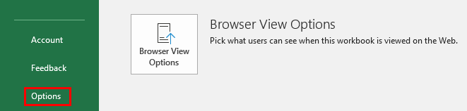
1. Step 1: First, we must enable the Analysis ToolPak Add-in.For this, click the “File” tab on the ribbon, and click the “Options,” once the file tab opens the below list.

    

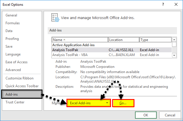
2. Step 2: On clicking “Options,” select “Add-ins” on the left side. Excel Add-ins are chosen in the “View and manage Microsoft Add-ins” and “Manage” boxes. Then, click “Go.”

   
   

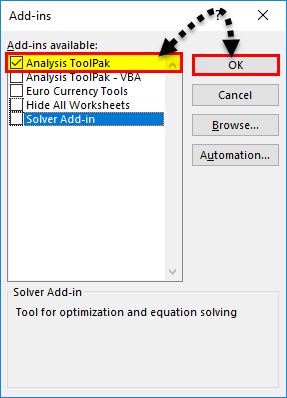
3. Step 3: In the Add-in dialog box, click on Analysis ToolPak, and click OK:

   
   
    

4. In the Add-in dialog box, click on Analysis ToolPak, and click OK:

   
   

   It will add the Data Analysis in Excel tools on the right-hand side to the Excel ribbon’s “Data” tab.
   
   

We can use the data for Regression Analysis in Excel, once the Analysis Toolpak is added and enabled in the Excel workbook.

We will see, with an example, how to use Regression Analysis in Excel.

Example #1

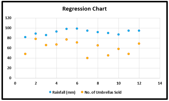
Consider the umbrellas sold data, with the months and rainfall, given in the image below.

The steps to perform the Regression Analysis in Excel are as follows:

• Step 1: On the Data tab in the Excel ribbon, click the Data Analysis

• Step 2: Click the “Regression” option, and click “OK” to enable the function.

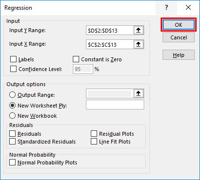
• Step 3: On clicking the “Regression” dialog box, we must arrange the accompanying settings:
  • For the dependent variable, select the “Input Y Range”, which denotes the dependent data. Here, in the below-given screenshot, we have selected the range from $D$2:$D$13.

• Select the “Input X Range,” which denotes the independent data for the independent variable. Here, in the below-given screenshot, we have selected the range from $C$2:$C$13.

• Step 4: Click “OK” and analyze the data accordingly.

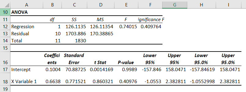
When you run the Regression Analysis in Excel, we will get the following output.

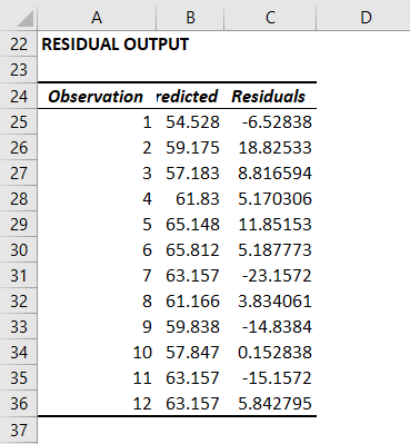
You can also make a scatter plot in excel of these residuals.

We will consider an example to create the Regression Chart In Excel.

The steps to Create Regression Chart in Excel are,

• Step 1: Select the data as given in the below screenshot.

• Step 2: Tap on the “Insert” tab. In the “Charts” gathering, tap the “Scatter” diagram or some other as a required symbol. Select the chart which suits the information.

• Step 3: We can modify the chart when required and fill in the hues and lines of your decision. For instance, we can pick alternate shading and utilize a strong line of a dashed line. We can customize the graph as we want to customize it.

We can calculate the Regression Using Excel Formula “y = bx + a”  

where,

• x – independent variable
• y – dependent variable
• a – y-intercept
• b – a slope of the regression line.

The steps to calculate the Regression Using Excel Formula are,

1. First, in a dataset, ensure we have all the values for the variables in the formula.
2. Next, in an empty cell, calculate the formula “y = bx + a” with the values.
3. Finally, when we press “Enter”, we get the output.

Once we get the output, we can plot the Regression Graph as we learned in the previous section, but this time including the output value cell too.

• We must always check the dependent and independent values to get an accurate output.
• When we test a huge number of data, we can thoroughly rank them based on their validation period statistics.
• Choose the data carefully to avoid any kind of error in excel analysis.
• We can optionally check any of the boxes at the bottom of the screen, although none of these is necessary to obtain the line best-fit formula.
• Start practicing with small data to understand the better analysis and run the Regression Analysis tool in Excel easily.

Regression analysis in Excel is a powerful tool to identify relationships between dependent and independent variables and make data-driven predictions. It’s easy to use with the help of the built-in tool Data Analysis Toolpak. Using it, you can gain valuable insights for business, research, or forecasting.