Formula with Text in Excel
Excel is a great tool for doing all the analysis and finalizing the report. But sometimes, calculation alone cannot convey the message to the reader because every reader has their way of looking at the report. Some people can understand the numbers just by looking at them, some need some time to get the real story, and some cannot understand. So, they need a full and clear-cut explanation of everything.
To bring all the users to the same page while reading the report, we can add text comments to the formula to make the report easily readable.
Let us look at how we can add text in Excel formulas.
#1 – Add Meaningful Words Using Text in Excel Formula
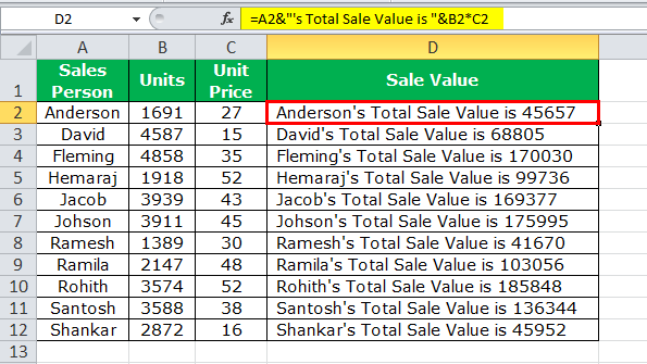
Often in Excel, we only perform calculations. Therefore, we are not worried about how well they convey the message to the reader. For example, take a look at the below data.

By looking at the above image, it is very clear that we need to find the sale value by multiplying Units to Unit Price.
Apply simple text in the Excel formula to get the total sales value for each salesperson.

Usually, we stop the process here itself.
How about showing the calculation as Anderson’s total “Sale Value” is 45,657?
It looks like a complete sentence to convey a clear message to the user. So, let us go ahead and frame a sentence along with the formula.
So, let us go ahead and frame a sentence along with the formula.
- We know the format of the sentence to be framed. Firstly, we need a “Sales Person” name to appear. So, we must select the cell A2 cell.

- Now, we need “Total Sale Value” after the salesperson’s name. We need to put the ampersand operator sign after selecting the first cell to comb this text value.

- Now, we need to do the calculation to get the sale value. Put on more (ampersand) sign and apply the formula as B*C2.

- Now, we must press the “Enter” key to complete the formula and our text values.
One problem with this formula is that sales numbers are not formatted properly. Because they do not have a thousand separators, that would have made the numbers look properly.There is nothing to worry about; we can format the numbers with the TEXT function in the Excel formula.Edit the formula. As shown below, the calculation part applies the Excel TEXT function to format the numbers.Now, we have the proper format of numbers along with the sales values. The TEXT function in Excel formula format the calculation (B2*C2) to the format of ###, ###.


#2 – Add Meaningful Words to Formula Calculations with TIME Format
We have seen how to add text values to our formulas to convey a clear-cut message to the readers or users. Now, we will be adding text values to another calculation, which includes time calculations.
We have data on flight departure and arrival timings. We need to calculate the total duration of each flight.

Not only the total duration, but we want to show the message like this “Flight Number DXS84’s total duration is 10:24:56.”
In cell D2, we must start the formula. Our first value is “Flight Number.” We must enter this in double-quotes.

The next value we need to add is the flight number already in cell A2. Enter the “&” symbol and select cell A2.

The next thing we need to add to the text‘s “Total Duration.”We must insert one more “&”symbol and enter this text in double-quotes.

Now comes the most important part of the formula. We need to calculate the total duration after “&” the symbol enters the formula as C2 – B2.

Our full calculation is complete. Press the “Enter” key to get the result.

We got the total duration as 0.433398, which is not in the right format. So, we must apply the TEXT function to perform the calculation and format that to TIME.

#3 – Add Meaningful Words to Formula Calculations with Date Format
The TEXT function can perform the formatting task when adding text values to get the correct number format. Now, we will see it in the date format.
Below is the daily sales table that we update the values regularly.

We need to automate the heading as the data keeps adding, i.e., we should change the last date as per the last day of the table.
Step 1: We must first open the formula in the A1 cell as “Consolidated Sales Data from.”

Step 2: Put the “&” symbol and apply the TEXT function in the Excel formula. Apply the MIN function to get the least date from this list inside the TEXT function. And format it as “dd-mmm-yyyy.”

Step 3: Now, enter the word to.

Step 4: To get the latest date from the table, we must apply the MAX formula, and format it as the date by using TEXT in the Excel formula.

As we update the table, it will automatically update the heading.
Things to Remember Formula with Text in Excel
- We can add the text values according to our preferences by using the CONCATENATE function in excel or the ampersand (&) symbol.
- To get the correct number format, we must use the TEXT function and specify the number format we want to display.
Recommended Articles
This article has been a guide on Text in Excel Formula. Here, we discuss how to add text in the Excel formula cell along with practical examples and downloadable Excel templates. You may also look at these useful functions in Excel: –