Compare And Match Columns In Excel

Last Updated :

Blog Author :

Edited by :

Reviewed by :

Table Of Contents

What Is Compare And Match Columns In Excel

Compare and column match is a function which is useful to match and compare the text in the given data. In excel we can compare data in single and two columns.

Consider the below table showing sample group in columns A and B.

Using EXACT function, let us compare and match two columns’ data.

So, the formula is =EXACT(A2,B2)

We can see the results in cell C2. Using autofill option, we can see the results in cells C3 and C4.

Likewise, we can use compare and match columns in Excel.

What Is Compare And Match Columns In Excel

Compare and Match two columns in Excel is a method used to compare and match data and find the results.
Comparing two columns in Excel for match can be done in different ways, depending on the user familiarity and data structure.
In Excel we can use this function depending on user preferences. Remember, for some reasons, we may need TRUE/FALSE results. Similarly, some users require and prefer personalized output.
Highlighting matching data or unique values is possible, and the matching process can be customized to meet user-specific needs.

How To Compare Two Columns In Excel For Match?

Comparing and matching two columns in Excel data can be performed in several ways depending upon the tools a user knows. It also depends on the data structure. For example, a user may want to compare or match two columns and get the result as TRUE or FALSE. Some users require the result in their own words. At the same time, some users want to highlight all the matching data. Some users want to highlight unique values. Like this, we can do the matching depending on the user's requirement.

Examples

Below are examples of matching or comparing two columns in excel.

Example #1 – Compare Two Columns of Data

For example, assume we have received city names from two different sources, sorted from A to Z. Below is the data set.

Follow the below steps:

We have city names from two different sources. We need to match whether "Source 1" data is equal to "Source 2" or not. Simple basic Excel formulas can do this. First, we need to open the equal sign in the C2 cell.
Since we match Source 1 = Source 2, let us select the formula as A2 = B2.
Then, press the "Enter" key. If "Source 1" is equal to "Source 2," we can get the result as "TRUE" or else "FALSE."
Next, we must drag the formula to the remaining cells to get the result.

In some cells, we received the result as "FALSE"(colored cells), which means "Source 1" data is not equal to "Source 2." Let us look at each cell in detail.

Cell C3: In the A3 cell, we have "New York," and in the B3 cell, we have "New York." Here, we do not have space characters after the word "New." So, the result is "FALSE."

Cell C7: In the A7 cell, we have "Bangalore," and in cell B7, we have "Bengaluru." So both are different. The result is "FALSE."

Cell C9: This is a special case. In cells A9 and B9, we have the same value as "New Delhi," but still, we got the result as "FALSE." It is an extreme case but a real-time example. By looking at the data, we cannot tell what the difference is; we need to go into minute analysis mode.
Let us apply the LEN function in Excel for each cell, which shows the number of characters in the selected cell.
In cell A9, we have 9 characters, but in cell B9, we have ten characters, i.e., one extra character. So then, we must press the F2 key (edit) in cell B9.
As we can see, one trailing space character entered after the word "Delhi" contributes as an extra character. To overcome these kinds of scenarios, we can apply the formula with the TRIM function, which removes all the unwanted space characters. Below is the way of using the TRIM function.

Now, let us look at the result in cell C9. We got the result as "TRUE" because we have applied a TRIM function. It has eliminated the trailing space in cell B9. Now, this is equal to cell A9.

Example #2 - Case Sensitive Match

If we want to match or compare two columns with a case sensitive approach, we need to use the Exact function in Excel.

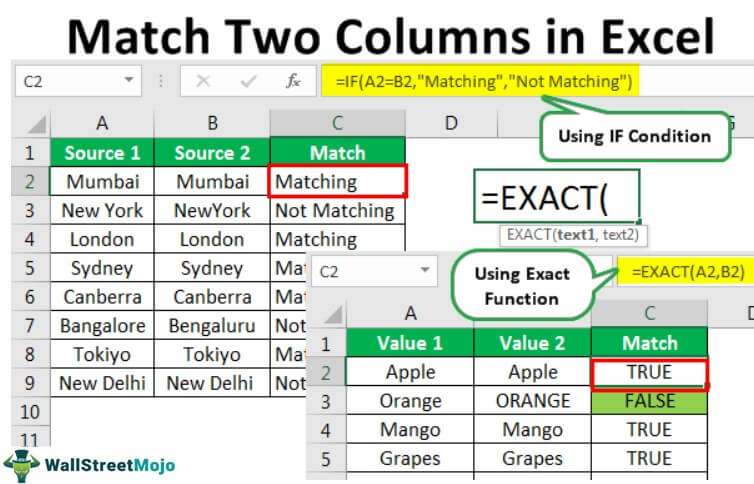
The EXACT function looks for two values and returns "TRUE" if the value 1 is equal to value 2. For example, if the value 1 is "Mumbai" and value 2 is "MUMBAI," it will return "FALSE" because the value 1 characters are in proper format and value 2 characters are in uppercase format.

Take a look at the below data now.

We have two values in the form of fruit names. Therefore, we need to match whether "Value 1" equals "Value 2."

Below is the EXACT formula.

Here, "Value 1" equals "Value 2," so it returns "True."

Then, drag the formula to other cells.

We have four values that are not exact.

Cell C3: In cell A3, we have "Orange," and in cell B3, we have "ORANGE." Technically both are the same since we have applied case sensitive match function in Excel. However, it has returned "FALSE."
Cell C7: Both the values are different in case matching: "Kiwi" and "KIWI."
Cell C8: In this example, only one character is case-sensitive: “Mush Milan” and “Mush Milan.”
Cell C9: Here, too, we have only one character case sensitive: "Jack fruit" and "Jack Fruit."

Example #3 - Change Default Result TRUE or FALSE with IF Condition

We have "TRUE" for matching cells and "FALSE" for non-matching cells in the above example. We can also change the result by applying the IF condition in excel.

If the values match, we should get "Matching," or we should call "Not Matching" as the answer by replacing default results of "TRUE" or "FALSE," respectively.

Let us open the IF condition in cell C3.

And enter the logical test as A2 = B2.

If the provided logical test in Excel is "TRUE", the result should be "Matching."

If the test is "FALSE," we need the result as "Not Matching."

Press the "Enter" key and copy-paste the formula to all the cells to obtain the result in all the columns.

So wherever data is matching, we get the result as “Matching,” or else we get the result as “Not Matching.”

Example #4 - Highlight Matching Data

With the help of conditional formatting, we can highlight all the matching data in excel.

We must select the data first and go to conditional formatting. Under conditional formatting, we must choose "New Rule."

Then, select "Use a formula to determine which cells to format." In the formula, the bar enters the formula as =$A2=$B2.

In the Format, the option chooses formatting color.

Click on "OK." It will highlight all the matching data.

Like this, we can match two columns of data in Excel in different ways.

Example #4 – Highlight Matching Data

Consider the below table showing the country names in columns A and B.

Using EXACT function, let us compare and match two columns’ data.

So, the formula is =EXACT(A2,B2)

We can see the results in cell C2.

Using autofill option, we can see the results in cell range C3:C6.

Important Things To Note

If the values match, we should output "Matching."
If not, output "Not Matching" by replacing the default results of "TRUE" or "FALSE."
When comparing two columns in Excel, the EXACT function should be used for case-sensitive matching.

Frequently Asked Questions

1. Can you use conditional formatting to compare two columns?

We can match data with ease using compare and match function in Excel. For example,

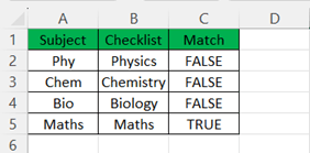
Consider the below table showing the subject list in columns A and B.

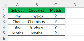
Using EXACT function, let us compare and match two columns’ data.

So, the formula is =EXACT(A2,B2) We can see the results in cell C2. Using autofill option, we can see the results in cell range C3:C5.

compare and match function in Excel - FAQ 1-1

To highlight matching data between two columns, you can use the duplicate function in conditional formatting. It's important to note that this process is distinct from comparing each row individually. When using this method, you won't be comparing each row one by one.

2. How do I compare two columns in Excel to remove duplicates?

To remove duplicate values from a range of cells, start by selecting that range. Before removing duplicates, make sure to remove any outlines or subtotals from your data. Next, go to the "Data" tab and click on "Remove Duplicates". Under the "Columns" section, select or deselect the columns where you want to remove the duplicates.

3. How do I remove duplicates from two columns match?

Removing duplicates in Excel is easy using the Remove Duplicates feature. Select the two columns that you want to remove duplicates from, and the feature will do the rest. Alternatively, you can manually combine the columns and then use Remove Duplicates on the resulting single column.