Index Match Multiple Criteria

We all use the Excel VLOOKUP function to fetch the data. Also, we know that the VLOOKUP function can bring the data from left to right, so the lookup value should always be on the left side of the result columns. However, we have several alternatives that can be used instead of the VLOOKUP function in Excel. 

We can use these INDEX + MATCH formulas to match multiple criteria for rows and columns with advanced technology. So, this article will take you through it in detail about this technique.

Here's a generic INDEX + MATCH formula to match multiple criteria in Excel:

=INDEX(return_range, MATCH(1, (criteria_range1=criteria1)*(criteria_range2=criteria2)*(criteria_range3=criteria3), 0))

Here,

• return_range – the range from which you want to return a value
• criteria_range1, criteria_range2, ... – ranges where criteria are applied and must be of the same length as the return range.

criteria1, criteria2, ... – the actual values to match in each respective range.

We explain using the INDEX+MATCH formula to match multiple criteria for rows and columns with examples.

Example #1 - INDEX + MATCH Formula

The majority of Excel users do not use lookup functions beyond the VLOOKUP function. The reasons could be so many, like its versatility and ease of use Let us briefly introduce this formula before going to the advanced level.

For example, look at the below data structure in Excel.

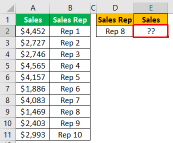
We have “Sales Rep” names and their respective sales values. Then, we have a drop-down list of “Sale Rep” in cell D2.

Based on our selection from the drop-down list, the "Sales" amount has to appear in cell E2.

We cannot apply the VLOOKUP formula because the lookup value “Sales Rep” is to the right of the result column “Sales.” So in these cases, we can use the combination INDEX + MATCH lookup value formula.

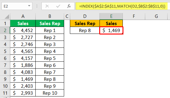
Step 1: Enter the following formula in cell E2.

=INDEX($A$2:$A$11,MATCH(D2,$B$2:$B$11,0)

1. The INDEX function looks for the mentioned row number value in the range A2:A11. 
2. Next, we have to provide the row from which we need the sales value. This row value is based on the “Sales Rep” value selected in cell D2. 
3. So the MATCH function looks for the “Sales Rep” row number in the range B2:B11 and returns the row number of the matched value.

Step 2: Press Enter. You get the sales value for the specified rep using INDEX-MATCH.

Example #2 - Multiple Criteria in INDEX + MATCH Formula

In this example, we have a data structure as seen below.

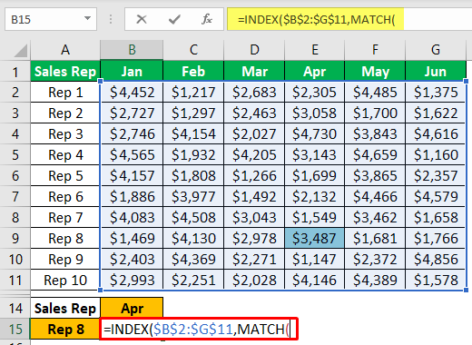
Step 1: We have monthly sales values of the representatives as “Sales Rep.” From this table, we need dynamic results like cell A15. So, we have created a “Sales Rep” drop-down list.

In the B14 cell, we have created a “Month” drop-down list.

Based on the selection made in these two cells, our formula has to fetch the data from the above table.

For example, if we choose “Rep 8” and “Apr,” then it has to show the sales value of “Rep 8” for the month of “Apr.”

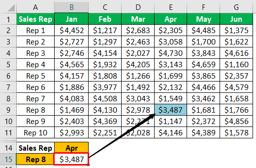
So, we need to match both rows and columns in these cases.

Step 2: Follow the below steps to apply the formula to match both rows and columns.

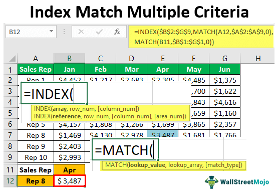
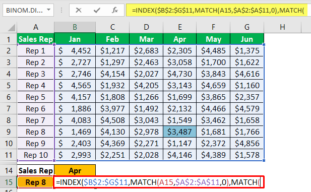
We must first open the INDEX function in cell B15.

Step 3: The first argument of the INDEX function is “Array,” i.e., from which range of cells we need the result. So, we need sales values in this case, so we must choose the range of cells from B2 to G11.

Step 4: The next argument of the INDEX function is from which row of the selected range we need the result. 

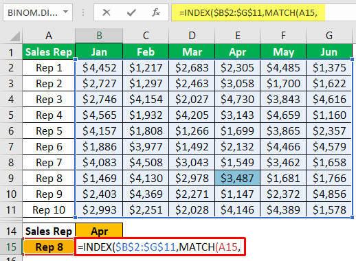
In this case, we need to arrive at the “Sales Rep” row number based on the selection made in the cell A15 drop-down cell. So, we must open the MATCH function for dynamically fetching the row number based on our selection.

Step 5: The lookup value of the MATCH function is “Sales Rep,” so we must choose the A15 cell as the reference.

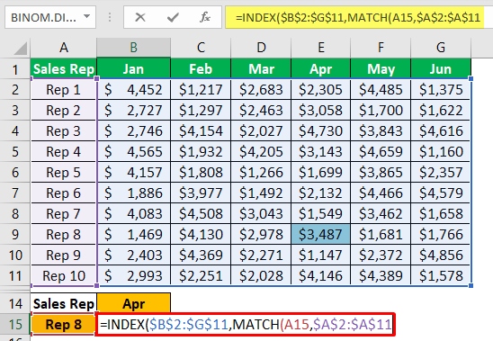
Step 6: The lookup array will be the “Sales Rep” named range in the main table. So, we must choose a range from A2 to A11.

Step 7: The MATCH type of the MATCH function will be exact. So, we must insert zero as the argument value.

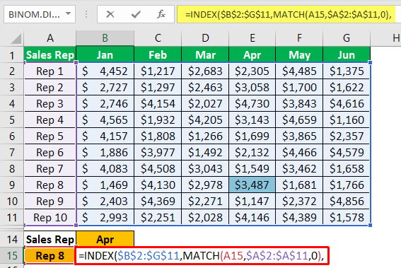
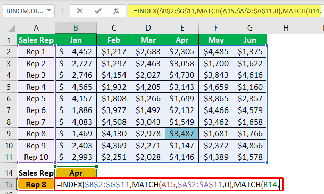
Step 8: The next argument of the INDEX function is “Column Number,” i.e., from the selected range of cells from which column we need the result. It is dependent on the month we choose from the drop-down list of cell B14. So, to get the column number automatically, we must open another MATCH function.

Step 9: The lookup value will be the month name, so select the B14 cell as a reference.

Step 10: The lookup array will be the month range of cells in the main table, i.e., B1 to G1.

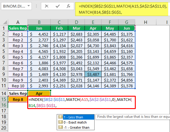
Step 11: The last argument is MATCH type. Choose “Exact Match” as the criteria. Close two brackets and press the "Enter" key to get the result.

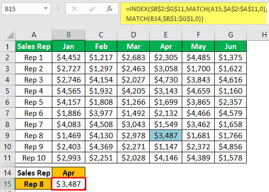
As we can see above, we have chosen “Rep 6” and “Apr” as the month, and our formula has returned the sales value for the month of “Apr” for “Rep 6”.

Note: Yellow-colored cell is the reference for you.

You can check out more on the INDEX MATCH combination in this INDEX MATCH article.

• Combining the Excel INDEX + MATCH function can be more powerful than the VLOOKUP formula.
• The INDEX and MATCH functions can match both rows and columns headers and return the result from the middle table.
• The MATCH function can return the row number and column number of the table headers of both rows and columns.