Table Of Contents
VLOOKUP Function
The VLOOKUP Excel function searches for a particular value and returns a corresponding match based on a unique identifier. A unique identifier is uniquely associated with all the records of the database. For instance, employee ID, student roll number, customer contact number, seller email address, etc., are unique identifiers.
For example, suppose you have a dataset of employee salaries ($150, $200, $500, $800 from B2:B5 and employee ID (1001,1002,1003,1004) from A2:A5. Then, in cell E2, we want to know the employee ID for the salary of $200, which is in cell B3. In such a scenario, we can use the VLOOKUP function. Then, inserting the lookup_value in cell D2, we can enter the formula as:
= VLOOKUP(D2,A2:B5,2,FALSE). It returns "1002"
In simple words, a user may use the VLOOKUP formula to search specific information (like employee ID) in an Excel database (table in Excel worksheet) and find information associated (employee's salary) with it.
The "V" in VLOOKUP stands for vertical. The function looks for a search value in the first column (lookup column) of the specified range and returns a match from the same row of another column (return column).
The VLOOKUP Excel function works for numerical, textual, and logical values. For example, an organization uses VLOOKUP to retrieve the monthly revenue of multiple products based on the product code (unique identifier).

The Syntax of the VLOOKUP Function
The syntax of the function is stated as follows:
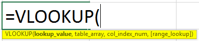
The function accepts four arguments: lookup_value, table_array, col_index_num, and range_lookup. The first three are mandatory arguments, while the last one is optional.
- lookup_value: Required. It represents the value we want to look for in the first column of a table or dataset.
- table_array: Required. It represents the dataset or data array that is to be searched.
- col_index_num: Required. It represents the integer specifying the column number of the table_array that we want to return a value from.
- range_lookup: Optional. It represents or defines what the function should return if it does not find an exact match to the lookup_value. This argument can be set to "FALSE" or "TRUE," where 'TRUE' indicates an approximate match (uses the closest match below the lookup_value in case the exact match is not found), and "FALSE" indicates an exact match (it returns an error in case the exact match is not found). "TRUE" can also be substituted for "1" and "FALSE" for "0."
VLOOKUP Excel Function - Explained in Video
How to Use VLOOKUP in Excel?
Let us go through a few examples of VLOOKUP in Excel. They will be beneficial for both beginners and advanced Excel users.
Example #1
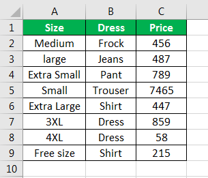
The following table shows the prices of various types of dresses. We want to find the price of the trouser, shirt, and dress.
Time needed: 2 minutes.
The steps to use the VLOOKUP Excel function are listed as follows:
First, organize the data in the left to right format because the function works in this order. Such an arrangement (shown in the next image) makes it easy to use the VLOOKUP function.
Place the cursor where the formula is to be entered. For example, since the trouser price is to be found, we place the cursor in cell F2, as shown in the next image.

Enter the formula "=VLOOKUP(E2,B1:C9,2,FALSE)". It is essential to supply correct arguments to the function to find the exact value.

In the following pointers (steps 3a to 3d), all the arguments of the VLOOKUP function concerning the current example are explained one by one.
Step 3(a): Lookup_value – This is the function's first and main argument. It specifies the value to be searched in the table. So, the "lookup_value" is E2 (trouser).
Step 3(b): Table_array-This refers to the table range in which the lookup value is to be searched. So, the lookup value is to be searched in the range B1:C9 of the lookup table.
Step 3(c): Col_index_num-This is the index number of the column. It specifies the column from which the value is to be returned. For example, the word "trouser" is present in column B (column 2).
So, this argument is 2, referring to the second column of the table array.
Note: The leftmost column of the table array is counted as 1.
Step 3(d): Range_lookup-This is the Boolean value "True" or "False." The values are explained as follows:
• True - It is used for an approximate or a close match. The data is matched with the argument approximately. For instance, the first word is looked up if the data contains more than one word.
• False - It is used for an exact match. All the words in the data are matched, and a corresponding value is returned.
Hence, we enter "False" because we want the formula to return an exact match. The complete formula is shown in the next image.
Note: If the "range_lookup" argument is omitted, the default value is "True."
Press the “Enter” key. All the arguments have been passed correctly. The result is displayed in the following image.

Drag the formula to obtain the prices of the shirt and dress. The output is shown in the following image.

Example #2
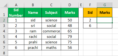
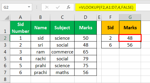
The following table shows the marks of 6 students in different subjects. The serial ID (Sid) number is in the first column (A).
We want to find the marks corresponding to serial ID numbers 2 and 6.
The steps to apply the VLOOKUP function are listed as follows:
Step 1: Organize the data and place the cursor in cell G2, where we will enter the formula.
Step 2: Enter the VLOOKUP Excel formula in cell G2. For auto-populating, the formula, press the "tab" key.
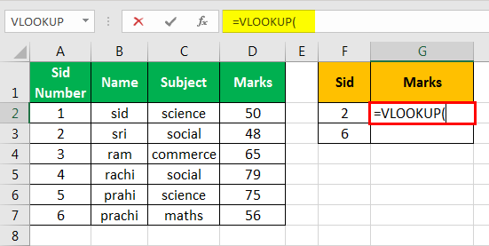
Step 3: Enter the function's first argument, as shown in the next image. The "lookup_value" is cell F2. It is the value we are looking for.

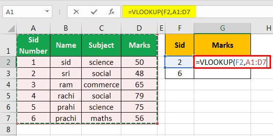
Step 4: Enter the next argument, the table_array. Select A1:D7 as shown in the following image. It is the source table where the serial ID is to be found.
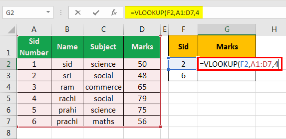
Step 5: Enter the col_index_num, the serial number of the column from which the value is to be returned. Since we want the function to return a value from the "marks" column, we type 4.
The serial ID number column (A) is counted as 1.
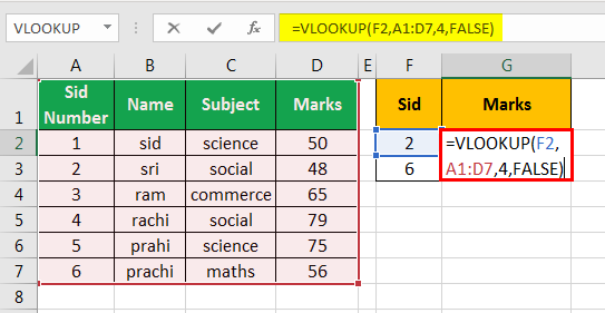
Step 6: Enter the argument "range_lookup," which consists of two values, "True" or "False." Since the latter value returns an exact match, we type "False." Finally, close the brackets of the formula.
The exact match option (False) is usually used to avoid confusion. The complete formula is shown in the following image.
Step 7: Press the "Enter" key as the formula is ready to be applied. The output is shown in the following image. Drag the formula of cell G2 to obtain the result in cell G3.
Example #3
The next table shows the names of 6 people along with their gender. The serial numbers are given in column A (Sno).
We want to find the serial number of a given gender.
The formula "=VLOOKUP(E2,A1:C7,1,FALSE)" returns the output #N/A error.
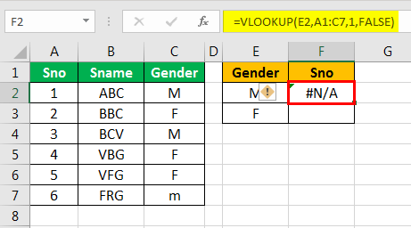
We want to find the serial number for the given gender. The lookup_value is E2 meaning the value to be looked up (gender) is to the right side of the serial number column (A).
The VLOOKUP function does not work because it looks for values beginning from left to right. Simply put, the lookup column (gender) should always be to the left of the return column (serial number or Sno).
The function searches the leftmost column of the "table_array" and returns a corresponding value from the right-hand side column.
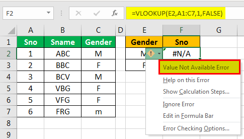
The #N/A error is the "value not available" error, as shown in the next image.
Note 1: The limitation of the VLOOKUP function in Excel is that it works on columns from left to right.
Note 2: Using the VLOOKUP to extract values from the left, is combined with the IF and CHOOSE functions.
The Characteristics of VLOOKUP Function
- It is not case-sensitive, implying that the uppercase and lowercase alphabets are treated the same.
- When duplicate values are absent, we should use them for a given data table. If duplicate matches are found, the function returns only the first one.
- It is often used in financial calculations.
The VLOOKUP Errors in Excel
The VLOOKUP formula returns errors on account for various reasons. There are three types of VLOOKUP errors which are explained as follows:
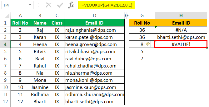
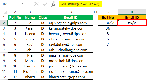
“#N/A!” error – This occurs if the function cannot find the "lookup_value" in the given "table_array."
“#REF!” error – This error occurs if the supplied col_index_ num argument exceeds the number of columns in the table_array.”
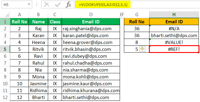
“#VALUE!” error – It occurs if the col_index_ num argument is not given or is supplied as less than 1.