What Is Strikethrough In Excel?
Strikethrough in Excel is a feature that strikes the selected cell values or puts a line between cells. If the cells have some values, the value has a line mark. It is a format in Excel that we can access from the “Format Cells” tab while right-clicking on it or from the Excel keyboard shortcut “CTRL + 1” from the numeric tab of the keyboard. The process is the same for removing a Strikethrough.
For example, we will apply Excel Strikethrough to cell A1, which has the value 123.
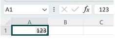
We get the output shown above, i.e., as 123.
Key Takeaways
- The Strikethrough in Excel helps users to strike any selected cell value, as a whole or a part of it, without changing the cell values, in the various methods.
- We can add a Strikethrough in simple ways, such as using the shortcut keys, i.e., “Ctrl+5”,
- adding the feature by creating a New tab, or in the Quick Access Toolbar, using Conditional Formatting, the Format Painter option, and a little more advanced way using the VBA Code.
- Irrespective of the methods we use to apply Excel Strikethrough Text, we can only use the shortcut key “Ctrl+5” to remove or delete the Strikethrough.
Top 6 Methods To Use Strikethrough In Excel
Below are the 6 methods to use Strikethrough in Excel.
- Using Excel Shortcut Key.
- Using Format Cell Options.
- Using from Quick Access Toolbar.
- Using it from Excel Ribbon.
- Using Dynamic Conditional Formatting.
- Using VBA.
Let us discuss each method in detail with an example.
Method #1 – Strikethrough Using the Excel Shortcut Key
The steps forStrikethroughusing theExcel shortcut keyare as follows:
- First, select the cells in which we need the Strikethrough format.

- Now, use the Excel Strikethrough shortcut key, “Ctrl+5”. The data will strike out, as shown below.


Method #2 – Strikethrough Using Format Cell Option
The steps to Strikethrough using Format Cell Option are as follows:
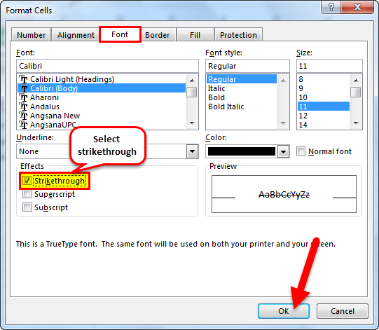
- Step 1: Select the cells that need this format, right-click on the cell, and choose the option of “Format Cells”.
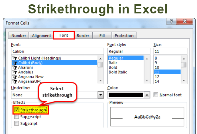
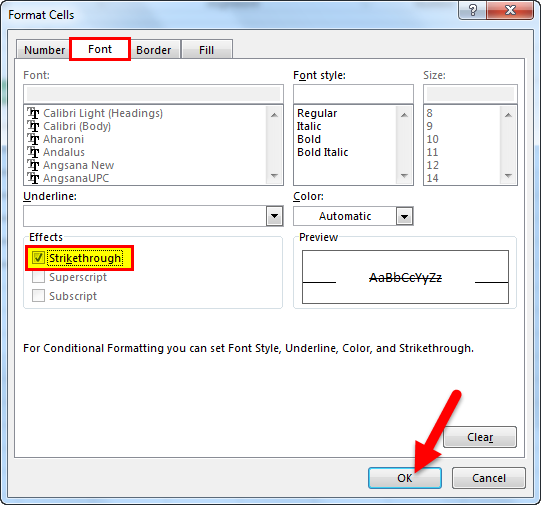
- Step 2: The “Format Cells” window opens. Here, go to the “Font” tab, check/tick the “Strikethrough” option, and click “OK.”
The output is shown below, i.e., the cells got the Strikethrough format.
Method #3 – Strikethrough using from Quick Access Toolbar
Let us add the option, as it is not available in the ribbon and in the Quick Access toolbar.
The steps to Strikethrough using from Quick Access Toolbar are as follows:
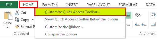
- Step 1: Right-click anywhere on the ribbon, and select the Customize Quick Access Toolbar.
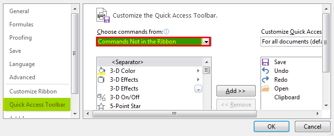
- Step 2: The “Excel Options” window appears.
- On the left, select the “Quick Access Toolbar” option.
- On the right, click the “Choose commands from:” option drop-down, and select the “Commands Not in the Ribbon” option.
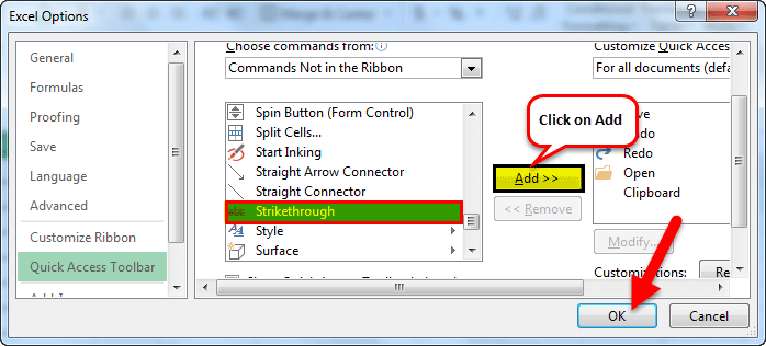
- Step 3: Next, select the “Strikethrough” command, click “Add,” and click “OK.”
- Step 4: After the option is added, it will appear on the “Title Bar”, as shown.
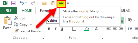
- Step 5: Select the data you want to Strikethrough, and click the “Strikethrough” option, as shown in the screenshot below.
- It will Strikethrough the selected cells, as shown below.
Method #4 – Strikethrough using it from Excel Ribbon
The steps to Strikethrough using it from Excel Ribbon are as follows:
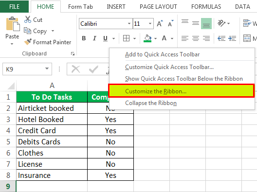
- Step 1: Right-click the “Font” tab, and choose the “Customize the Ribbon” option.
- Step 2: The “Excel Options” window appears.
- On the left, select the “Quick Access Toolbar” option.
- On the right, click the “Choose commands from:” option drop-down, and select the “Commands Not in the Ribbon” option.
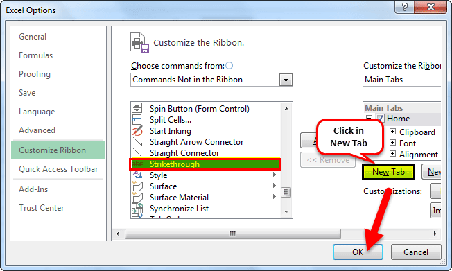
- Finally, select the “Strikethrough” option, click “New Tab,” and click “OK.”
- Step 3: After the option is added, a “New Tab” tab appears in the ribbon, with only the “Strikethrough” group, as shown below.
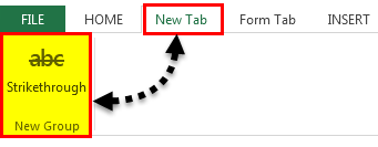
Step 4: Finally, select the cells you want to Strikethrough – go to the “New tab” tab – click the “Strikethrough” from the “New Group”. The output is shown below.
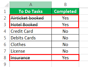
Method #5 – Strikethrough using Dynamic Conditional Formatting
- Step 1: Choose the range where we want to apply the conditional formatting, click the “Conditional Formatting” option drop-down in the “Home” tab’s “Styles” group, and then click the “New Rule”, as shown below.
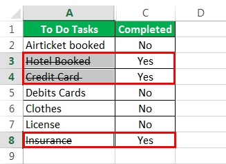
- Step 2: Click on “Use a formula to determine which cells to format”, insert the formula as (=B2=” Yes”), and then click “Format.”

Step 3: The “Format Cells” window appears. Here, go to the “Font” tab, check/tick the “Strikethrough” option, and click “OK.”
Step 4: After the Conditional Formatting, Excel will automatically strike out the text, as shown below.
Method #6 – Strikethrough Using VBA
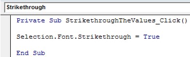
We will create a Strikethrough command button using VBA.
The steps to Strikethrough using VBA are as follows:
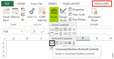
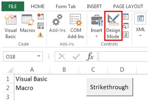
- Step 1 – Choose the “Command button” from the “Insert” command available in the “Controls” group under the Developer tab excel.
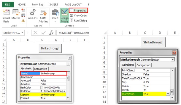
- Step 2 – Create the command button, and change the “Properties”, as shown in the images below.
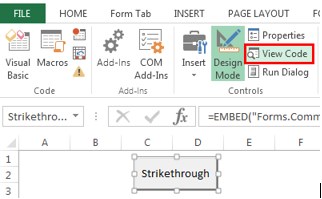
- Step 3 – Click “View Code” from the “Controls” group after closing the properties dialog box. (Ensure the button is selected and “Design Mode” is activated.)
- Step 4 – Choose “Strikethrough” from the list.

Now, paste the following VBA code.
- Step 5 – Save the file with .xlsm
Suppose we want to Strikethrough two cells (A1 and A2). We can do the same by selecting the cells and pressing the command button (make sure the “Design Mode” is deactivated).
Select the cells, and click the button, to get the following output.
Important Things To Note
- Strikethrough, when applied, does not change the value of the cell. For example, “TEXT” is the same as “
TEXT” for Excel and formulas. - If we only want a certain part of the cell value to Strikethrough, we must select that part instead of the complete cell.
- If we are using Conditional Formatting for Strikethrough, we should keep in mind that the reference of the range must not be an absolute or a relative range reference.
- While adding the shortcut of the strike, we should keep in mind that we cannot edit the tabs that Excel creates. We cannot add this option to the “Font” tab, as this is a default tab that we cannot edit in any way.
Frequently Asked Questions (FAQs)
Where is option Strikethrough Text in Excel?
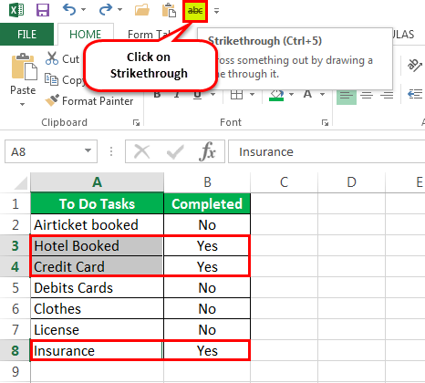
Unlike MS Word, we do not have the Strikethrough in Excel in the Font group, by default. Therefore, we use the feature as follows:
a. Click the “Format Cells” launcher, shown by the yellow arrow.
b. The “Format Cells” window opens.
c. Under the “Font” menu, check/tick the “Strikethrough” checkbox in the “Effects” option.
d. Click “OK”.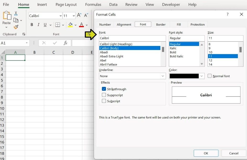
What methods open the Format Cells window to Strikethrough in Excel?
There are various methods to open the Format Cells window, namely,
• Method 1 – Simply press the shortcut key “Ctrl+1”.
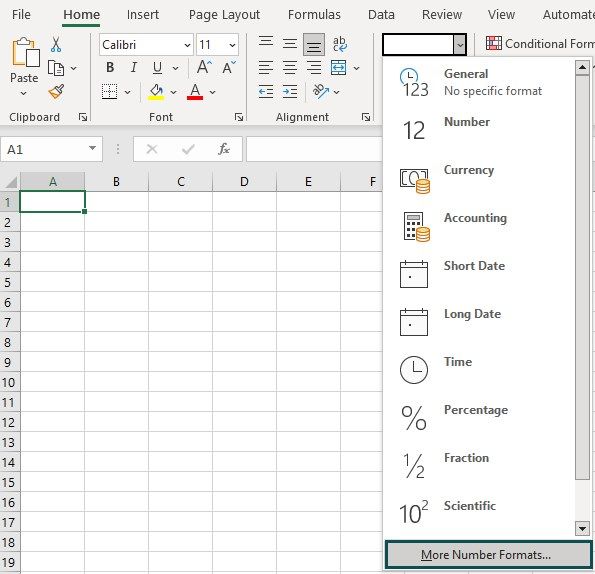
• Method 2 – Select the “Home” tab – go to the “Number” group – click the “Number Format” option drop-down – select the last option “More Number Formats…”, as shown below.
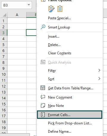
• Method 3 – Right-click on any cell, and select the “Format Cells…” option from the list, as shown below.
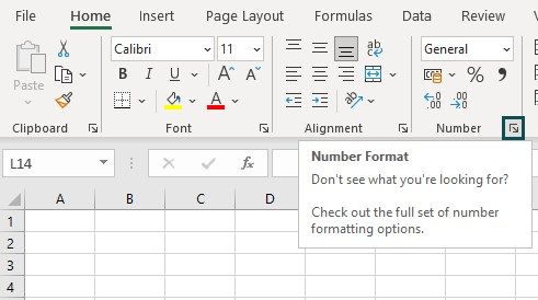
·• Method 4 – Select the “Home” tab – go to the “Number” group – click the “Number Format” box, i.e., the small box at the bottom right of the “Number” group, as shown below.
Is there an Alternate way to Strikethrough in Excel?
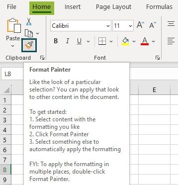
Yes, there is an alternate way to convert decimal values to Strikethrough in Excel using the “Format Painter” option.
For example, when we have multiple cell values to Strikethrough,
• First, select the cell value which has already has a Strikethrough format.
• Next, select the “Home” tab – go to the “Clipboard” group – click the “Format Painter” option to copy the cell formatting, as shown below.
• Finally, paste it to the cell with another cell value without the Strikethrough formatting. Repeat the same with the other cells too.
Recommended Articles
This article has been a guide to Strikethrough in Excel. Here we use Strikethrough using shortcut, QAT, customize ribbon, VBA, examples, downloadable excel template. You may learn more about Excel from the following articles: –