Table Of Contents
IFERROR With VLOOKUP To Get Rid Of #NA Errors
The IFERROR function is an error handling function, and the VLOOKUP function is a referencing function. These functions are combined and used so that when the VLOOKUP function encounters an error while finding or matching the given data, we can provide a solution. The VLOOKUP function is nested in the IFERROR function.
To get rid of an #N/A error when using VLOOKUP, wrap the formula with IFERROR.
Key Takeaways
- Combining the VLOOKUP with the IFERROR function helps replace different errors like #DIV/0 and #N/A with alternatives, such as an alternative result and message.
- It helps improve the readability of your spreadsheet by removing the visible error codes.
- IFERROR works with all types of errors and is available in Excel 2007 and newer versions.
Examples
The IFERROR function in Excel handles errors such as #N/A, #VALUE!, or #DIV/0! in formulas. When it is combined with VLOOKUP, it allows you to display a custom message when a lookup fails, which makes our spreadsheets cleaner. Let us look at some simple examples on this topic.
Example #1
Table 1 is the main data source. Table 2 is the VLOOKUP table. We have applied a VLOOKUP formula to find the sales amount for laptop brands in column F.

In the above table, we got an error for Apple and Notepad's brands as they are not present in Table 1. We can fix this issue by using the IFERROR function with the VLOOKUP function.
- Step 1: We must apply the IFERROR function before the VLOOKUP function in Excel. We need to write the Vlookup formula inside the IFERROR formula.
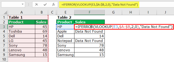
=IFERROR (VLOOKUP (E3, $A: $B, 2, 0),"Data Not Found")
Firstly, the IFERROR function tries to find the value for the VLOOKUP formula.
Secondly, If the VLOOKUP function does not find a value, it will return an error. Therefore, if there is an error, we will show the result as "Data Not Found."
- Step 2: by applying the formula in Table 2, we have replaced all the #N/A values with the "Data Not Found" text. Definitely, this will look better than the #N/A.

Example #2
Not only can we use the IFERROR function with the VLOOKUP function in Excel. We can use this with any other formula too.
Look at the below example where we need to calculate the variance percentage. If the base value is, the missing calculation returns the error as #DIV/0!

So, we can apply the IFERROR method here to eliminate such errors as #DIV/0!

If any given calculation returns any error, the IFERROR returns the result as 0%. If there is no error, then the normal count will happen.
Manual Method to Replace #N/A Or Any Other Error Types
However, we can replace errors with the IFERROR formula. There is one manual method: the FIND and REPLACE method.
- Step 1: Once the formula is applied, copy and paste only values.

- Step 2: Press "Ctrl + H" to open, replace the box, and type "#N/A" If the error type is #N/A.

- Step 3: Now, we must write the "Replace with" values as "Data Not Found."

- Step 4: Click on the "Replace All" button.

It would instantly replace all the #N/A values with "Data Not Found."

Note: If we have applied a filter, we must choose the "Visible cells only" method to replace.
Want to learn in detail about LOOKUP functions in Excel? Consider going ahead with our LOOKUP functions course in Excel.
Things To Remember
- The IFERROR function can make the numerical reports beautiful by removing errors.
- If the data contains an error type and if we apply PivotTables, then the same kind of error will occur in the PivotTable too.
- Though we can use the IFNA formula, it is not flexible to give results for errors other than #N/A.
- In Excel 2007 and earlier versions, the formula to get rid of the #N/A error is an ISERROR.