Find and Replace in Excel

Last Updated :

Blog Author :

Edited by :

Reviewed by :

Table Of Contents

What is Find and Replace Feature in Excel?

The Find and Replace feature of Excel looks for a data value and replaces it with another data value. This data value can be a text string, number, date or special character. The Find and Replace feature can search within a worksheet or workbook, by rows or columns, and within formulas, values or comments.

For example, in a financial report of Excel, the text string “asset” may need to be replaced with “assets.”

The purpose of using the Find and Replace feature in Excel is to locate certain information in a database. It also allows modifying the existing data values with a few clicks. By default, the Find and Replace excel feature looks for a partial match. But, it can also look for an exact match if the option “match entire cell contents” is selected.

What is Find and Replace Feature in Excel?

How to Access the Find and Replace Feature of Excel?

The shortcuts to the Find and Replace excel feature are stated as follows:

“Ctrl+F” opens the Find tab of the Find and Replace feature.
“Ctrl+H” opens the Replace tab of the Find and Replace feature.

Alternatively, the “find” and “replace” options can be clicked from the “find & select” drop-down (“editing” group) of the Home tab. These options open the Find and Replace tabs of the Find and Replace feature of Excel.

Let us consider some examples to understand the working of the Find and Replace feature of Excel.

Example #1–Find a Partial Match in a Worksheet

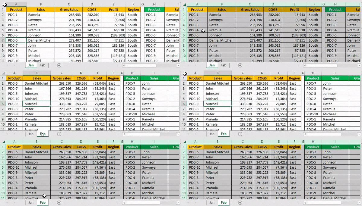
The following image shows two worksheets titled “Jan” and “Feb.” These worksheets contain datasets that report the sales made (column C) to different customers (column B) in January and February.

The names of the products, cost of goods sold (COGS), profits, and regions are also displayed in columns A, D, E, and F respectively. A similar dataset (with different numbers) is in columns H to M as well.

Find the name “Mitchel” in the worksheet “Jan.” Use the Find and Replace feature of Excel.

The steps to use find and replace function in excel is follows:

Go to the worksheet “Jan.” Next, press the keys “Ctrl+F” together. The Find tab of the “find and replace” dialog box opens. This is shown in the following image.

Note: By default, Excel searches in the currently active worksheet.
Type the word to be searched in the “find what” box. We type “Mitchel.”

Note that this search is not case-sensitive. So, even if the worksheet contains “MITCHEL,” it will show up in the search results.
Press either the “Enter” key or the “find next” option. The first occurrence of the name “Daniel Mitchel” is selected. So, cell B7 is selected, as shown in the following image. Clicking “find next” again and again selects the subsequent occurrences of “Mitchel.”

Notice that though we entered “Mitchel” in the “find what” box, Excel has selected the name “Daniel Mitchel.” This is called a partial match. It implies that if there are any additional words preceding or succeeding the search value, the entire string containing the search value is returned in the result.
Click “find all” to see all the strings containing “Mitchel.” The results are shown in the following image. These results display the following information:

• The column “book” displays the name of the workbook containing the search value.
• The column “sheet” displays the name of the worksheet containing the search value.
• The column “cell” displays the reference of the cells containing the search value.
• The column “value” displays the entire string containing the search value.

Notice that at the bottom of the dialog box, Excel displays the number of cells containing the search value. In this case, there are 8 cells in the worksheet “Jan,” which contain either “Mitchel” or “Daniel Mitchel.”

Difference between “find all” and “find next”: The “find all” option shows all the occurrences of the search value. Further, clicking any of the entries shown by this option takes the user to the corresponding cell.

The “find next” option helps scan through the different cells containing the search value. Clicking “find next” for the first time selects the first occurrence of the search value. Likewise, clicking “find next” the second time selects the second occurrence of the search value, and so on.

Example #2–Find a Partial Match in a Workbook

Working on the dataset of example #1, find the name “Mitchel” in the entire workbook. Use the Find and Replace feature of Excel.

The steps to search the stated string in the entire workbook are listed as follows:

Step 1: Press the keys “Ctrl+F” together. The Find tab of the “find and replace” window opens. Type the name “Mitchel” in the “find what” box.

Next, click “options,” shown within a black box in the following image.

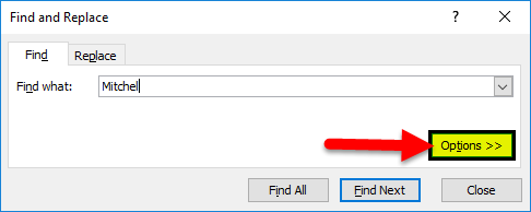
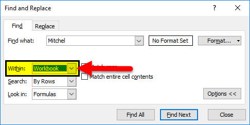
Step 2: Clicking “options” expands the “find and replace” dialog box. Click the drop-down next to the option “within” and select “workbook.”

The selection is shown in the following image.

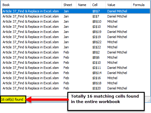
Step 3: Click “find all” to see all the results. The results are shown in the following image. This time the string “Mitchel” has been found in 16 cells of the workbook.

Clicking any of the entries will select the respective cell.

Example #3–Find an Exact Match in a Workbook

Working on the dataset of example #1, find an exact match of “Mitchel” in the entire workbook. Use the Find and Replace feature of Excel.

The steps to search the exact name in the entire workbook are listed as follows:

Step 1: Press the keys “Ctrl+F.” In the Find tab of the “find and replace” window, perform the following tasks:

Click “options” to expand the “find and replace” window.
Enter the name “Mitchel” in the “find what” box.
Select “workbook” in the box adjacent to “within.”
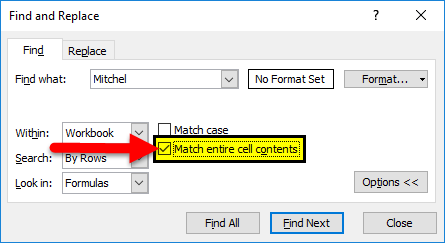
Select the checkbox of “match entire cell contents.”
Leave the “search” and “look in” parameters to default values which are “by rows” and “formulas” respectively.

The name of the “find what” box and the selections are shown in the following image.

Note: When the option “match entire cell contents” is selected, the Find and Replace excel feature looks for exactly those data values that have been entered in the “find what” box.

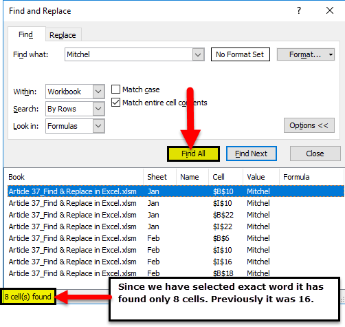
Step 2: Click “find all” to view all the exact matches of the name “Mitchel.” In the current workbook, 8 cells contain the exact name.

The results (shown in the following image) display the cell references, exact value, and the names of the worksheet and the workbook.

Example #4–Replace the Range Reference of a Formula

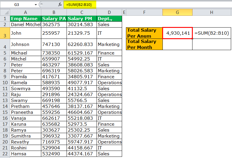
The following image shows the names (column A), salaries per annum (in $ in column B), salaries per month (in $ in column C), and departments (column D) of some employees of an organization.

The total salary per annum is shown in cell G3. This sum incorrectly considers the range B2:B10 in place of the range B2:B22. Rectify the range of the formulas in cells G3 and H3 so that the total salary per annum is calculated accurately. Use the Find and Replace feature of Excel.

The steps to edit a formula by using the Find and Replace feature of Excel are listed as follows:

Step 1: Copy the SUM formula of cell G3. For this, perform the given tasks:

Select cell G3. The formula appears in the formula bar.
Copy this formula by pressing the keys “Ctrl+C” together.
Press the Escape (Esc) key once the formula has been copied. This will help exit the formula bar.

Alternatively, copy the formula of cell H3 by pressing the keys “Ctrl+C.” Next, press “Ctrl+H.”

Step 2: The Replace tab of the “find and replace” window opens. Paste the copied formula in the “find what” box, as shown in the following image. For pasting the formula, press the keys “Ctrl+V” together.

Note: Instead of copying and pasting, one can type the formula directly in the “find what” box.

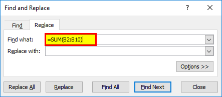
Step 3: Enter the correct formula in the “replace with” box. So, type the formula “=SUM(B2:B22)” without the beginning and ending double quotation marks. This is shown in the following image.

Next, click “replace all.”

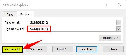
Step 4: Click “Ok” in the message stating the number of replacements made. The formulas of cells G3 and H3 change from “=SUM(B2:B10)” to “=SUM(B2:B22).” As a result, the total salary per annum changes.

The new output is shown within a red box in the following image. Hence, the total salary paid to the given 21 employees is $11,179,954 per annum.

Example #5–Replace the Existing Text to Make Two Strings Identical

There are two images titled “image 1” and “image 2.” Both images are in different worksheets. Further, the following information is given:

Image 1 shows the product code (column A) and prices (in $ in column B) of 21 products of a multinational organization.
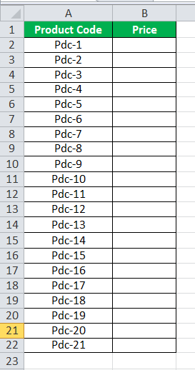
Image 2 shows the product code (column A) and a blank column (column B) for the prices of the 21 products.

Notice that the product codes of both images consist of some letters prefixed to a number. The letters are different in both images, but the subsequent numbers are the same.

Make the product code identical in both images by using the Find and Replace feature of Excel. This will help fetch the prices of “image 1” in “image 2” (column B) with the VLOOKUP function.

Image 1

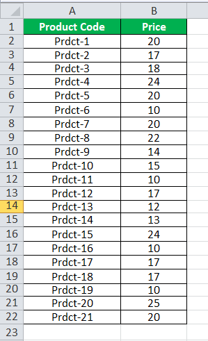
Image 2

The steps to make the product code identical by using the Find and Replace feature of Excel are listed as follows:

Step 1: Press the keys “Ctrl+H” to open the Replace tab of the “find and replace” window.

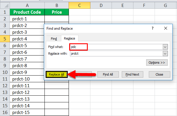
Step 2: Enter “pdc” in the “find what” box. Enter “prdct” in the “replace with” box. Next, click “replace all.” A message stating the number of replacements made is displayed. Click “Ok” to proceed.

The entries and the outputs are shown in the following image. Now, one can easily apply the VLOOKUP function to fetch the prices in this image. Had the replacements not been made, the VLOOKUP function could not have been applied.

Difference between “replace all” and “replace”: The “replace all” option replaces all the occurrences of the search value in one go. In contrast, the “replace” option replaces one occurrence at a time.

Therefore, use “replace” when not sure which occurrence needs to be replaced. Use “replace all” when all occurrences of the search value need to be replaced.

Example #6–Replace the Old Formatting of a Cell

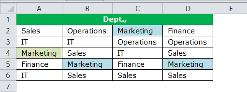
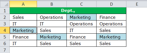
The following image shows some departments of an organization. Cell A4 is in grey and cells B5, C2, and D5 are in blue. We want all the cells containing “marketing” to be in one color.

Therefore, replace the grey color of cell A4 with blue color. Use the Find and Replace feature of Excel.

The steps to change the formatting with the Find and Replace feature of Excel are listed as follows:

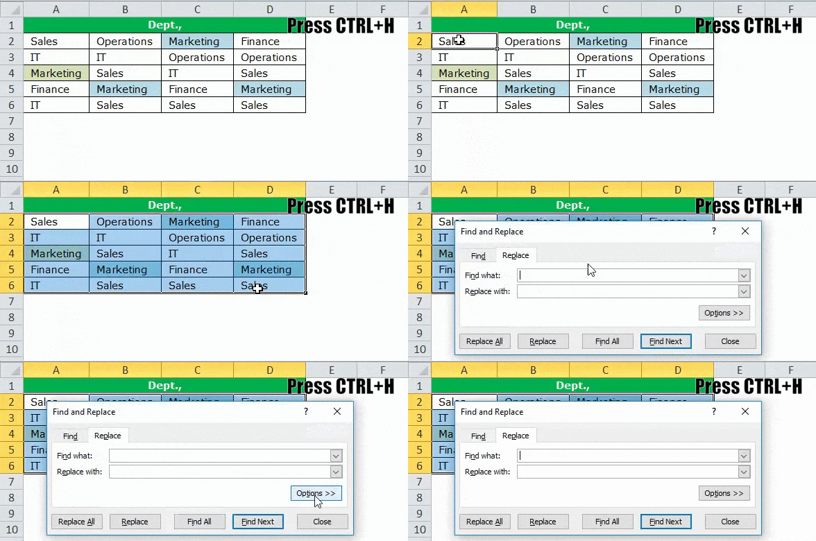
Step 1: Select the dataset whose formatting needs to be changed. We have selected the range A2:D6.

Next, press the keys “Ctrl+H” to open the Replace tab of the “find and replace” window. In this tab, click “options” shown on the right side.

This entire step is shown in the following image.

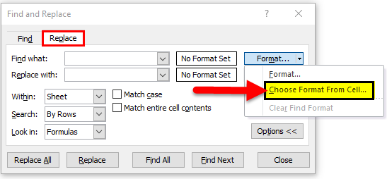
Step 2: Once “options” is clicked, the “find and replace” window expands. Click the drop-down arrow of the first “format” option (to the right of the “find what” box). Next, select “choose format from cell.”

The selection is shown within a black box in the following image.

Step 3: Select the cell whose formatting needs to be changed. We select cell A4. As a result, the “no format set” on the left of “format” changes to “preview.” This “preview” option reflects the color of cell A4, as shown in the following image.

Note: The “preview” option of the following image and cell A4 of the first image (at the beginning of this example) show a slight variation in color. Please ignore this variation, which may be due to different Excel versions being used to create images.

Step 4: Click the drop-down arrow of the second “format” option (to the right of the “replace with” box). Select “choose format from cell” and click any of the blue cells (B5, C2 or D5). Consequently, the “preview” option appears in blue, as shown in the following image.

Next, click “replace all.”

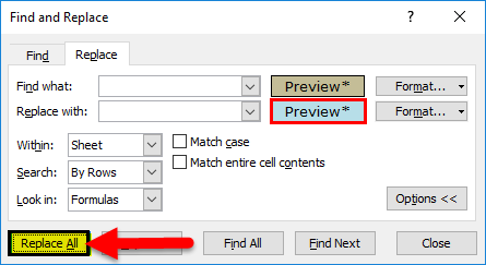
Step 5: Excel shows the number of replacements made. Click “Ok” to proceed. The output is shown in the following image.

Hence, cell A4 has also been colored blue. In this way, the formatting of a cell can be searched and replaced. So, we have searched for the grey color and replaced it with the blue color. Now, all cells containing “marketing” are in a single color.

Note: Alternatively, one can select the “format” option from both the “format” drop-downs. Thereafter, from the respective “fill” tabs, select the color to be searched and the color to be replaced with.

Example #7–Find a Comment in a Worksheet

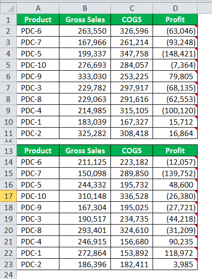
The following image contains two datasets (range A1:D11 and range A13:D23) that show the gross sales (column B), cost of goods sold (COGS in column C), and profits (column D) of ten products of an organization. Further, the following information is given:

Both datasets pertain to different time periods. The figures in brackets in column D are the losses suffered by the organization.
In both datasets, each cell of column D contains comments. This is indicated by the small, red triangles at the top-right side of each cell.
There are three kinds of comments, namely, “no commission,” “commission @ 5%,” and “commission @ 10%.”

Find the comment “no commission” in the current worksheet, which has been renamed “comment.” Use the Find and Replace feature of Excel.

The steps to search a specific comment by using the Find and Replace feature of Excel are listed as follows:

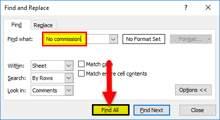
Step 1: Open the Find tab of the “find and replace” dialog box. For this, press the keys “Ctrl+F” together. Next, click “options.” Make the following selections in this window:

Select “sheet” and “by rows” in the “within” and “search” parameters. These are the default selections of Excel.
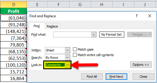
Select the option “comments” from the drop-down of “look in.”

The selection of the second pointer is shown within a black box in the following image.

Step 2: In the “find what” box, enter the string of the comment that needs to be searched. We have entered “no commission,” as shown in the following image.

Next, click “find all.”

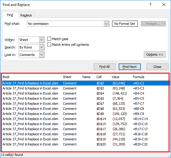
Step 3: The search results are shown in the following image. Notice that 13 cells (refer to the bottom of the image) contain the comment “no commission.”

The references to cells containing the specific comment (no commission) are displayed in the column “cell.” The formulas (of column D) and the names of the workbook and worksheet are displayed in columns “formula,” “book,” and “sheet” respectively.

Clicking any of the entries of these results will select the cell containing the comment.

Frequently Asked Questions

1. Define the Find and Replace feature and state how it is used in Excel.

The Find and Replace feature of Excel helps search a data value and replace it with another data value. The need to search a data value arises when certain information is to be located in a database. The need to replace a data value arises when the existing information requires to be changed.

The Find and Replace feature (or window) of Excel can be used in either of the following ways:

• Use the Find tab when a data value needs to be searched. Specify the data value in the “find what” box and click “find next” or “find all” to search.
• Use the Replace tab when one data value needs to be replaced by another. Specify the value to search and the value to replace with, in the “find what” and “replace with” boxes respectively. Click “replace” or “replace all” to make the replacements.

Note: Click the “options” button to view more features of the “find and replace” window of Excel.

2. How to use the Find and Replace feature with wildcards in Excel?

The Find and Replace feature can be used with the wildcard characters like an asterisk (*), question mark (?), and tilde (~) in the following ways:

• The asterisk looks for any number of characters. For instance, “ro*” will find the strings rose, product, root, metro, rhinoceros, and so on. So, the words having “ro” anywhere in the string will be returned in the search results.
• The question mark looks for a single character of the string. For instance, “s?m” will find the strings simplicity, sampling, similarity, blossom, troublesome, and so on. So, the words having any character between “s” and “m” (placed anywhere in the string) are returned in the search results.
• The tilde looks for the actual asterisk, question mark or tilde in the strings. For instance, “~?” will find “happy?,” “mer?ry,” “?joyful,” “cheerful?”, and so on. So, the words having a question mark anywhere in the string are returned in the search results. Likewise, “~*” and “~~” look for words that contain asterisk or tilde at any place in the string.

The wildcard characters stated in the preceding pointers need to be typed in the “find what” box. The value to be replaced with needs to be entered in the “replace with” box.

Note: To look for an exact match, select the option “match entire cell contents.”

3. How is the Find and Replace feature used for the following tasks of Excel?

1. Replace a value with nothing
2. Assign a format to specific cells

1. The steps to replace a value with nothing are listed as follows:

a. Open the Replace tab by pressing the keys “Ctrl+H.”
b. Type the value to be replaced with nothing in the “find what” box.
c. Leave the “replace with” box blank.
d. Click the “replace all” button.

All occurrences of the value typed in the “find what” box are deleted.

2. The steps to assign a format to specific cells are listed as follows:

a. Open the Replace tab by pressing the keys “Ctrl+H.”
b. In the “find what” box, type the text string to be formatted.
c. In the “replace with” box, type the same text string as that of the preceding step.
d. Click “options.” The “find and replace” window expands.
e. Click the “format” drop-down to the right of “replace with.” Select the option “format.” The “replace format” window opens.
f. Assign the desired formatting in the “alignment,” “font,” “border,” and “fill” tabs.
g. Click “Ok” in the “replace format” window. Click “replace all” in the “find and replace” window. Click “Ok ” in the message stating the number of replacements made.

The new formatting will be assigned to the cells containing the “find what” string. Notice that no replacements of data values will be made. This is because the text of “find what” and “replace with” boxes are the same. So, there is only a change in the formatting of specific cells.