ISFORMULA Function

What Is ISFORMULA Excel Function?

The ISFORMULA function in Excel is a built-in Information function. It accepts a cell reference, formula, or a name referencing a cell and determines whether the referenced cell contains a formula or not. If the specified cell contains a formula, the ISFORMULA function output is TRUE; otherwise, it is FALSE.

Users can utilize the ISFORMULA() to identify cells containing formulas in massive financial and statistical datasets, which helps in error checking and troubleshooting.

For example, the dataset below shows a list of values in column A, and the methods used to update the values in the column A cells are shown in column B.

The requirement is to determine whether the cells in column A contain formulas and display the output as logical values, TRUE or FALSE, in column C.

Then, we can obtain the required output using ISFORMULA function in each target cell.

In the above ISFORMULA function in Microsoft Excel example, the ISFORMULA() in each target cell accepts the reference to the respective column A cell.

The ISFORMULA function then checks if the specified cell contains a formula. It returns TRUE if the cell value is a formula output and FALSE otherwise.

Furthermore, we can corroborate the ISFORMULA function output in the target cells with the corresponding column B cells. Column B shows which column A cells contain formulas and those which contain values.

• The ISFORMULA function enables one to check if a cell contains a formula or not. While the function input can be a cell reference, a formula, or a name referencing a cell, the function output will be TRUE if the referenced cell contains a formula. Otherwise, the function output will be FALSE.
• Users can utilize the ISFORMULA Excel function to locate cells containing formulas in massive datasets, which makes error detection and correction more straightforward.
• The ISFORMULA Excel function accepts one mandatory argument, reference.
• While we can utilize the ISFORMULA() as a standalone function, using it with other inbuilt functions, such as IF and FORMULATEXT, helps achieve fruitful results.

Syntax

The ISFORMULA function in Microsoft Excel syntax is as follows:

Where,

• reference: This is the reference to the cell we aim to test for a formula using the ISFORMULA function. It is a mandatory argument, typically a cell reference, formula expression, or a name referencing a cell.

Please note that if the reference argument value is of an invalid data type, the Excel ISFORMULA function output will be the #VALUE! error value.

How To Use ISFORMULA Function In Excel?

Though we can use the Excel VBA ISFORMULA function, the following two methods are the more straightforward options to utilize the function:

1. Access from the Excel ribbon.
2. Enter into the worksheet manually.

Method #1 - Access From The Excel Ribbon

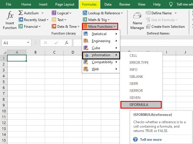
Select a cell for output - choose the Formulas tab - click the More Functions group functions down arrow - click the Information group functions right arrow - select the Excel ISFORMULA function, as depicted below.

The Function Arguments window will appear. Enter the mandatory function argument in the Reference field.

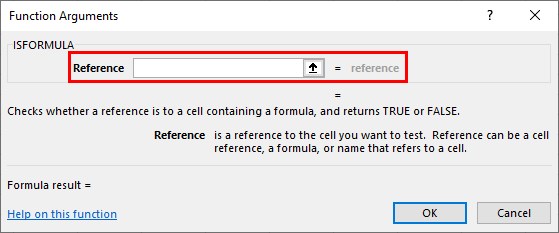
Click OK in the Function Arguments window to close it and obtain the required ISFORMULA function output in the chosen cell.

Method #2 - Enter Into The Worksheet Manually

1. Choose a cell for the output.
2. Type =ISFORMULA( in the cell.
3. Enter the cell reference, formula expression, or a name referencing a cell as the argument value.
4. Close the brackets and press Enter to view the ISFORMULA function output, a logical value, in the chosen cell.

Examples

Check out the following ISFORMULA function examples to use the function effectively.

Example #1 - Highlight Cells With A Formula

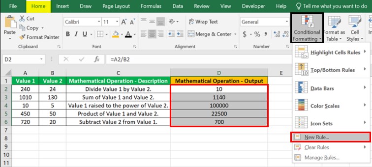
The dataset below contains two sets of values in columns A and B. Column C shows the descriptions of the mathematical operations required to be performed with the values in each row. On the other hand, column D shows the corresponding mathematical operations’ results based on the descriptions.

The requirement is to highlight cells containing formulas in column D range D2:D6.

Then, we can achieve the desired output using ISFORMULA function in the Excel Conditional Formatting feature.

Step 1: Select the range D2:D6 and choose Home - Conditional Formatting - New Rule.

The New Formatting Rule window will appear, where we must choose the last rule type to use the ISFORMULA function as a formula to evaluate the cells to highlight.

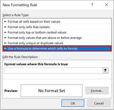
Step 2: Enter the ISFORMULA() as the formula to format values when the formula is true.

=ISFORMULA(D2)

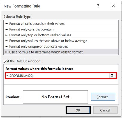
Next, select Format.

Step 3: The Excel Format Cells window will appear. Click the Fill tab to open it and choose the color to highlight the cells where the specified ISFORMULA() formula is true.

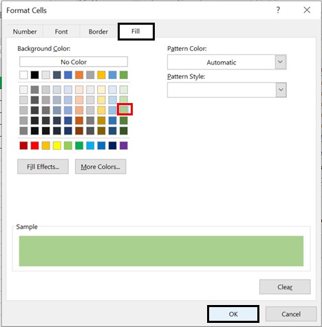
Click OK.

Step 4: Click OK in the New Formatting Rule window.

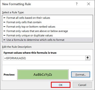
The window will close, and the column D cells containing formulas will appear highlighted in the chosen color.

The ISFORMULA function checks each cell, in the range D2:D6, whether it contains a formula. The function output is TRUE when a cell has a formula and FALSE otherwise.

Next, the Conditional Formatting feature highlights the cells where the ISFORMULA() output is TRUE in the chosen shade.

Thus, the output shows that cells D2, D4, and D6 contain formulas, and the values they display are the formulas’ outputs. On the other hand, cells D3 and D5 contain values. So, they remain not highlighted.

Example #2 - Test A Cell For A Formula

The image below shows two datasets.

While the first one lists students and their test scores in different subjects, the second shows a student and their score in the specified subject, based on the first dataset. And the score in the second dataset is in cell H2.

The task is to determine if cell H2 contains a formula and display the output in cell I2.

While we can use the Excel VBA ISFORMULA function, the following steps show the simpler methods to achieve the required outcome.

Step 1: Choose cell I2, enter the ISFORMULA function, and press Enter.

=ISFORMULA(I2)

Example #3 - Using ISFORMULA With A Range Of Cells

The image below contains a list of items and their order dates, expected to be updated using the Excel DATE function.

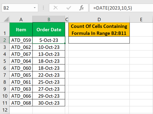
The requirement is to determine the total count of cells in the range B2:B11 that contain formulas and display the output cell D2.

Then, we can use the ISFORMULA function in the Excel SUM function in the target cell and obtain the required count.

Step 1: Choose cell D2 and enter the SUM() containing the ISFORMULA().

=SUM(--ISFORMULA(B2:B11))

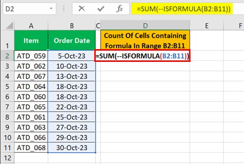
Step 2: Press Ctrl + Shift + Enter to execute the expression as we would implement array formulas in Excel.

{=SUM(--ISFORMULA(B2:B11))}

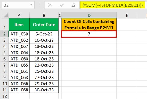
First, the ISFORMULA() returns an array of TRUEs and FALSEs, based on the range B2:B11 values, {TRUE;TRUE;FALSE;TRUE;TRUE;TRUE;FALSE;TRUE;TRUE;FALSE}. The TRUEs indicate the corresponding cells in the specified range contain formulas. On the other hand, FALSEs indicate the corresponding cells in the specified range do not contain formulas.

Next, the double unary operator helps convert the logical TRUEs and FALSEs into 1s and 0s. Finally, the SUM() adds the elements of the resulting array, {1;1;0;1;1;1;0;1;1;0} to return the value 7 as the required count of cells containing formulas in the range B2:B11.

Example #4 - Show Formula, If Cell Contains One

The following dataset lists a set of values in column A.

The requirement is to check if the column A cells contain formulas. If they do, display the formula in the corresponding column B cells and the "No Formula” message if they do not.

Then, the steps are as follows:

Step 1: Choose cell B2, enter the required ISFORMULA function-based formula, and press Enter.

="Formula in cell "&CELL("address",A2)&": "&IF(ISFORMULA(A2), FORMULATEXT(A2), "No Formula")

We shall split the cell B2 formula into three sections to understand the logic. While the first two are to show a text in the target cell, the third part is crucial in determining the output we require.

First, the Excel CELL function returns the address of the specified cell, which is A2, as an absolute reference, $A$2.

Next, the ISFORMULA() is the Excel IF function condition. It checks if cell A2 contains a formula. Since the cited cell contains one, the ISFORMULA() output is TRUE. Thus, the IF() returns the TRUE value, which is the FORMULATEXT function. So, the FORMULATEXT() returns the cell A2 formula as a string.

Finally, the formula concatenates the text, the CELL() output, and the IF() output to return the required output.

Step 2: Using the Excel fill handle, update the formula in the remaining target cells.

Please note that if the column A cell does not contain a formula, the ISFORMULA(), as the IF() condition, in the corresponding target cell returns FALSE. Thus, the IF() condition does not hold, and the phrase “No Formula” appears in the target cell.

Important Things To Note

• Ensure the reference argument value is of the valid data type in the ISFORMULA function. Otherwise, the function return value will be the #VALUE! error in Excel.
• If the cell referenced in the ISFORMULA Excel function contains a formula returning an error value, then the ISFORMULA() will return logical TRUE as the output.

Frequently Asked Questions (FAQs)

Download Template

This article must be helpful to understand the ISFORMULA Function, with its formula and examples. You can download the template here to use it instantly.

Recommended Articles

This has been a guide to What Is ISFORMULA Function. Here we learn the ISFORMULA function syntax & how to use it in Excel with examples & points to remember. You can learn more from the following articles –

• Basic Excel VBA Course
• Excel Protect Formulas
• Evaluate Formula in Excel