Ribbon In Excel

The ribbon is an element of the UI (User Interface) at the top of Excel. In simple words, the ribbon can be called a strip consisting of buttons or tabs seen at the top of the Excel sheet. The ribbon was first introduced in Microsoft Excel in 2007.

In an earlier version of Excel, a menu and toolbar were replaced by a ribbon 2007. The basic tabs under the ribbon are – "Home," "Insert," "Page Layout," "Formulas," "Data," "Review," and "View." We can customize it according to the requirements. See the image below. The highlighted strip is called ribbon, consisting of tabs like "Home, "Insert," etc.

1. The ribbon in Excel is a user interface strip located at the top of the sheet. It consists of buttons and tabs and was introduced in 2007.
2. Add only frequently used tabs to the ribbon to improve performance. Place logical commands in logical groups or tabs for easy access.
3. When adding commands from the "Command" option, ensure that a "New Group (Custom)" has been created. Otherwise, an error will be displayed. When adding commands, ensure that a "New Group (Custom)" is created, or it will display an error.

Ribbons are similar to the catalogue of options and functions we can use in Excel. To understand effectively, we need to understand how to

• Hide Ribbons
• Show or unhide ribbons
• Customize ribbons

In this article, we will learn all 3 with detailed examples.

We can easily hide ribbons in Excel with the following ways;

• Use the shortcut key, Ctrl + F1.
• We can also double click on the tab we are currently in to hide the entire ribbon.
• Similarly, we can also click on the pin seen on the lower-right corner and select the option, Show Tabs Only to hide the ribbon.

We can easily unhide or show ribbons in Excel with the following ways;

• Use the shortcut key, Ctrl + F1.
• We can also double click on the tab we are currently in to hide the entire ribbon.

Below are the steps to customize the ribbon.

Step 1 - Right-click anywhere on the ribbon. It will open a pop-up with options, including “Customize the Ribbon.”

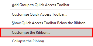
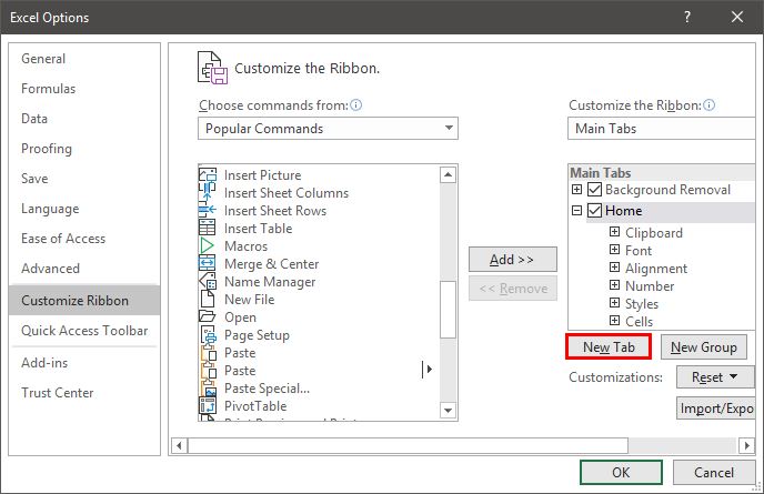
Step 2 - This will open the Excel Options box for you.

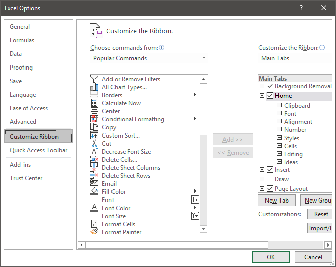
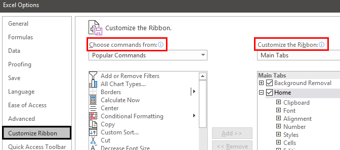
Step 3 - You can see two options on the screen: “Customize the Ribbon” on the right and the “Choose commands from” option on the left.

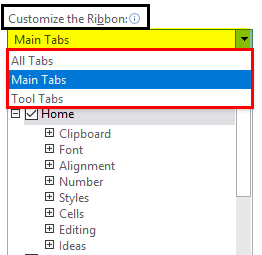
In the dropdown below, there are three options to customize the ribbon. By default, the “Main Tabs” is selected. The other two are "Tool Tabs" and "All Tabs."

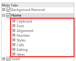
Step 4 - You can click on the (+) sign to expand the list.

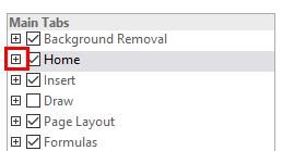
You will see some more tabs under the "Main Tabs."

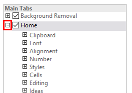
You can shrink the list by clicking on the (-) sign.

Step 5 - You can select or deselect the required tab to customize the ribbon. It will appear on the sheet accordingly.

You can also add additional tabs to your sheet by following the below steps.

• Click "New Tab (Custom)" or "New Group (Custom) " and rename it with some name (not necessary) by clicking on the "Rename" option.

• Choose a command from the option and select the desired option from the dropdown.
• Add command to the tab or group you have created.

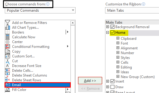
Note: You can also open the Excel option pop-up by following the steps.

Click on File Menu ---> Options

It will open Excel options for you, where you will see the option to customize the ribbon.

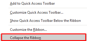
You can collapse the ribbon by right-clicking anywhere on the ribbon and then selecting the "Collapse the Ribbon" option.

Below are some examples where you required customization of the ribbon.

Example #1

Someone asks you to record a macro or write a code in VBA. How will you do that?

Solution:

We can use excel shortcuts "Alt + F8" to record macro and "Alt + F11" to open the VBA screen. But remembering shortcuts is not always easy, so here is another option.

Shortcut key to Record Macro:

Shortcut key to Open VBA Screen:

Add the "Developer" ribbon in Excel by using the following steps. 

First, “Customize the Ribbon” will open the Excel options box.

Check the "Developer" option shown in the list under the “Main Tabs.” See the image below. Click "OK."

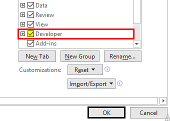
You will see the developer tab under the ribbon. See the image below.

You can see the macros or basic visual screens option.

Example #2

Someone asks you to create an interactive dashboard using Power View in Excel 2016.

Solution:

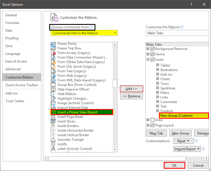
The "Power View" option is hidden in Excel 2016. So, we must follow the below steps to add the "Power View" command in our Excel. First, go to "Customize the Ribbon."

Under "Customize the Ribbon," extend the "Insert" option, then click on the "New Group (Custom)."

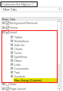
Now, choose the command shown on the left and select the command, not in the ribbon from the dropdown. Now, select "Insert a Power View Report." Next, click on "Add." It will add a "Power View" under the "Insert" tab. (When you click on "Add," make sure a "New Group (Custom)" is selected. Else, an error will pop up). Select "OK." See the below image:

Now, you can see the "Power View" option under the "Insert" tab in the "New Group" section:

Example #3

Let us take another scenario.

Suppose we are working on a report requiring the sum of the values in subsequent rows or columns very frequently.

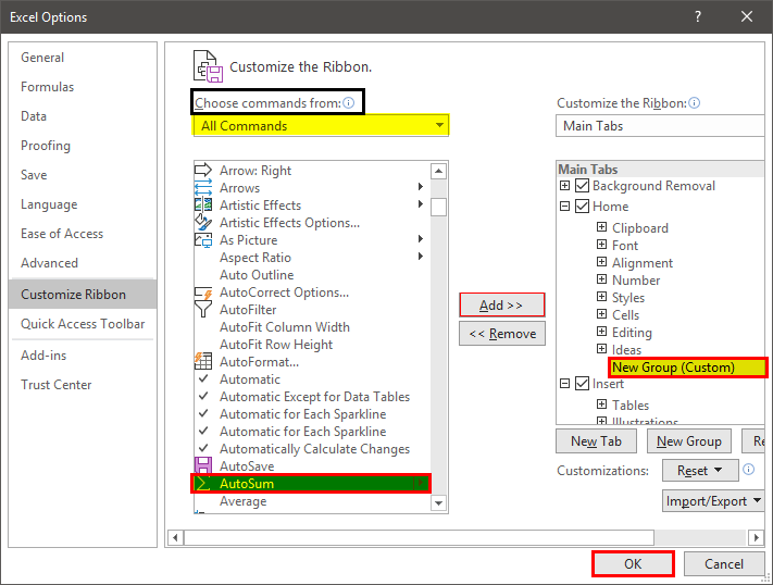
To sum up the values, we need to write a SUM function whenever the total value is required. Here, we can simplify our work by adding the AutoSum command to our ribbon. Then, go to "Customize the Ribbon."

Under "Customize the Ribbon," extend the "Home" tab, then click on the "New Group (Custom)."

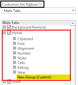
Now, choose the command shown on the left and select “All commands” from the dropdown. Now, select the "∑" AutoSum option. Next, click on "Add." It will add "∑" "AutoSum" under the "Home" tab. (when you click on "Add," make sure a "New Group (Custom)" is selected. Else, an error will pop up). Select "OK." See the below image:

Now, you can see the "AutoSum" option under the "Home" tab in the "New Group" section:

Now, let us see its use.

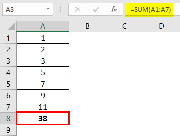
We have some numbers in cells A1 to A7. We need to get the sum in A8. Select cell A8 and click "AutoSum." It will automatically apply the SUM formula for the active range and give you the SUM.

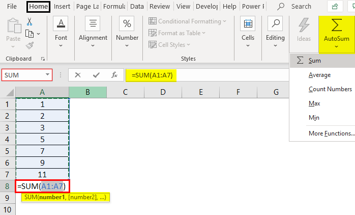
We get the following result.

• We must slow the performance by adding tabs to the ribbon. So, we must add and keep only those tabs, whichever is required frequently.
• We must add a logical command to a logical group or tab so it can easily find that command.
• When adding commands from the "Command" option, not the ribbon, we must ensure that we have created a "New Group (Custom)." Otherwise, it will display the error.

This article is a guide to Ribbon in Excel. Here, we discuss how to customize, collapse, and use ribbon in Excel, along with examples and explanations. You can learn more about Excel from the following articles: -

• List of Top 10 Excel Commands
• Step Chart work in Excel
• Watermark in Excel
• Excel 2016 Ribbons