Two-Variable Data Table in Excel

How to Create a Two-Variable Data Table in Excel?

Two-variable data table helps us to analyze how the combination of two different variables impact on the overall data table. The word itself suggests two variables involved in this data table. In simple terms when the two variables change what is the impact on the result. In one variable data table, only one variable changes but here two variables change simultaneously.

Examples

Let us take some examples to see how we can create a two-variable data table in excel.

Example #1

Assume that you are taking a loan from the bank and are in discussion with the bank manager regarding your interest rate and the repayment period. You need to analyze at the different interest rates and at different repayment periods what is the monthly EMI amount you need to pay.

Also, assume that you are a salaried person, and after all your monthly commitments, you can save a maximum of Rs. 18 500/-.

The initial proposal forms the bank is as bellows.

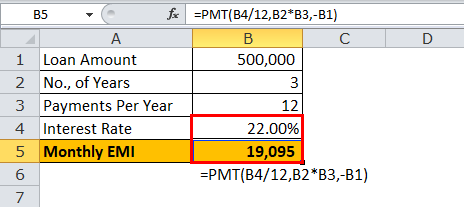
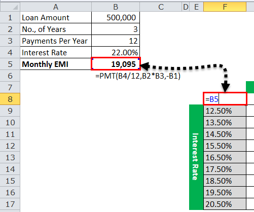
At a 22% PA interest rate, the monthly EMI for 3 years is 19,095.

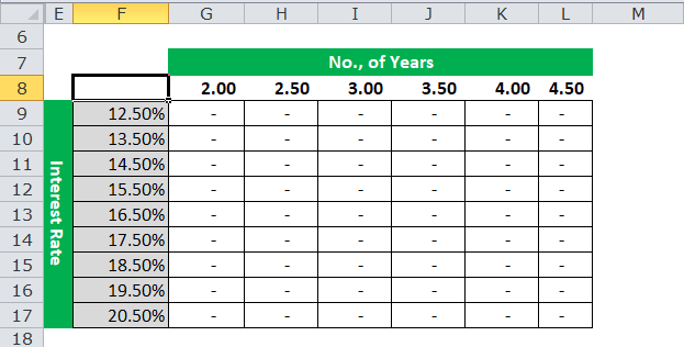
Create a table like this.

Now to the cell F8, give a link to the cell B5 (that contains EMI calculation).

Select the data table that we have created for creating scenarios.

Go to Data, then select What if Analysis and Data Table.

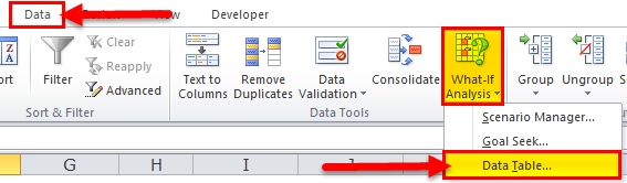
Now click on Data Table. It will open up the below dialogue box.

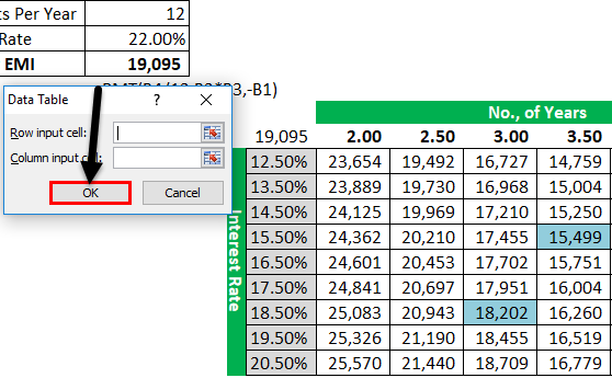
We have arranged our new tables like different interest rates vertically and different years horizontally.

In our original calculation, the interest rate is in the cell B4, and the number of years cell is in the cell B2.

Therefore, for row input cell give a link to B2 (that contains years and in our table years are there horizontally) and for column input cell give a link to B4 (that contains interest rate and in our table interest rate is there vertically)

Now click on, OK. This would create a scenario table instantly.

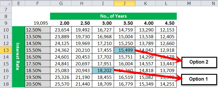
So now, you have all the scenarios in front of you. Your monthly savings is 18500 per month.

Option 1: If you do not want some spare cash.

You need to negotiate with the bank for an interest rate of 18.5% per anum for 3 years. If you can negotiate for this rate, you need to pay a monthly EMI of Rs. 18202.

Option 2: If you need some spare cash.

In this volatile world, you need some cash all the time. So cannot spend all the 18500 savings money for your salary.

If you want to let us say 3000 per month as spare cash, you need to negotiate with the banker for a maximum of 15.5% for 3.5 years. In this case, you need to pay a monthly EMI of 15,499 per month.

Wow!! Such a useful tool we have in excel. We can analyze and choose the plan or idea according to our wishes.

Example #2

Assume you are investing money in mutual funds through SIP planning. Monthly you are investing in 4500. You need to make an analysis to know what the return on an investment after certain years is.

You are not sure when to stop investing money and what is the percentage you are expecting.

Below are the basic details to do the sensitivity analysis.

Particulars	Amount
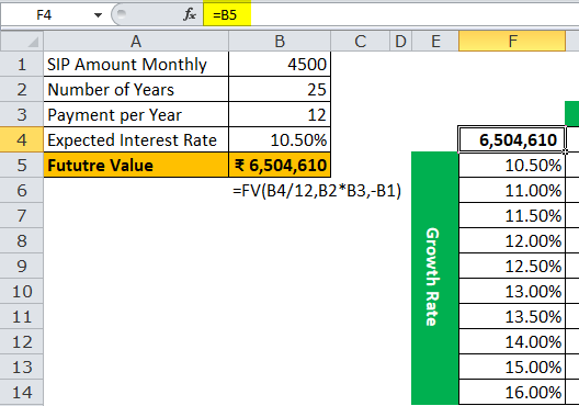
SIP Amount Monthly	4500
Number of Years	25
Payment Per Year	12
Expected Interest Rate	10.50%
Future Value	???

Apply FV function to know the future value after 25 years of investment.

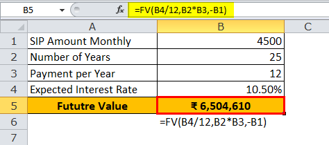
Ok, the future value of your investment after 25 years is 65 lakhs.

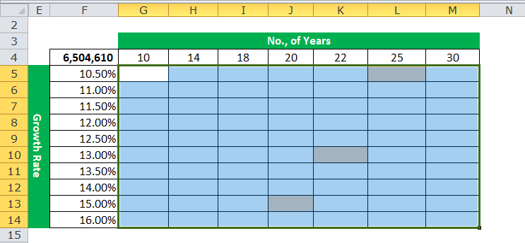
Now you need to know at different years and at different rates what would be the return on investment. Create a table like this.

Now give a link to the cell F4 from B5 (which contains the future value for our original investment).

Select the table we have created.

Go to Data, then select What if Analysis and Data Table.

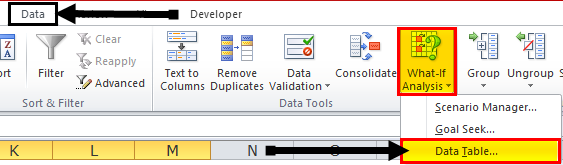
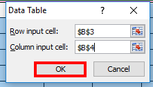
Now click on Data Table. It will open up the below dialogue box.

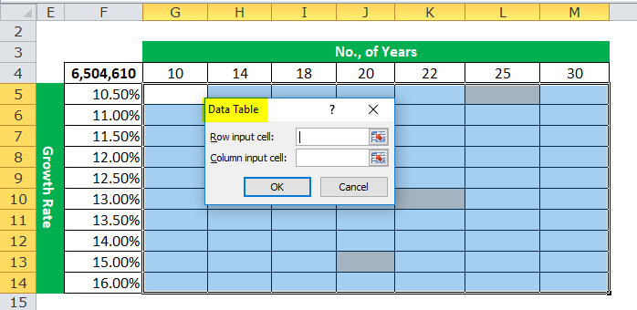
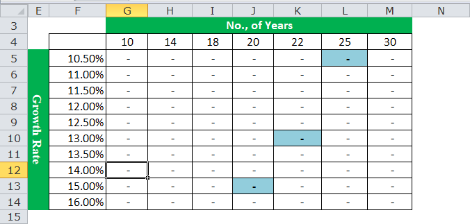
In the ROW, input cell select give the link to the cell B2 (that contains no., years). The reason why we have selected this cell because we have created a new table, and in that table, our years in the row format, i.e., horizontally.

In the COLUMN, input cell select give the link to the cell B4 (that contains the expected return percentage). The reason why we have selected this cell because we have created a new table, and in that table, our expected percentages are in column format,i.e., vertically.

Click on Ok this will create a scenario table for you.

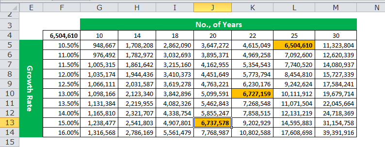
Look at the cells that I have highlighted. In the first attempt, we need to wait for 25 years to get the sum of 65 lakh at a 10.5% return. However, at a 13% return rate, we get that amount in 22 years. Similarly, at a 15% return rate, we get that amount in just 20 years.

These how we can do a sensitivity analysis by using the two-variable data table in excel.

Things to Remember

• We cannot undo the action (Ctrl + Z) taken place by the data table. However, you can manually delete all the values from the table.
• We cannot delete once cells at a time because it is an array formula.
• The data table is a linked formula, so it does not require manual updating.
• This is very helpful to look at the result when two variables changes at a time.

Recommended Articles

This has been a guide to creating Two-Variable Data Table Excel. Here we discuss how to create a Two-Variable Data Table Excel using examples and downloadable excel templates. You may also look at these useful excel tools –

• How to use PPMT Function in Excel?
• Excel Data Table
• MS Excel Course
• One-Variable Data Table Excel
• CSV Files into Excel