Brownian Motion In Finance

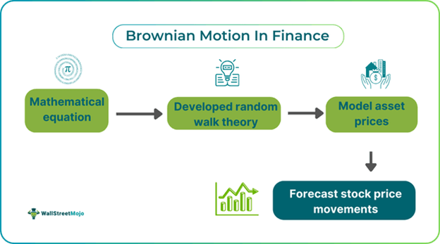
Brownian motion in finance is used to model asset prices, such as stocks trading in financial markets. The concept was initially introduced in botany, emphasizing the random movement of pollen particles, but it was later applied to study asset price behavior. It can be used for different financial instruments, such as stocks, derivatives, option pricing, and so on.

In an active market session, stock price movements generally depict a random pattern. Asset prices fluctuate every second due to several market factors and forces, such as inflation, liquidity, industry news, press releases, company valuation, volatility, demographics, global events, and supply and demand. All these factors contribute to making price movements vary, and market participants try to anticipate stock prices.

Brownian motion in finance is the equation that allows investors to study the behavior of asset prices to forecast future stock prices based on past and current prices. It can be anything from stocks, derivatives, option pricing or any other underlying asset. The concept was initially introduced by a botanist, Robert Brown, in 1827 when he was observing the pollen particles’ random movement due to water molecules with the help of a microscope. Later, in the 1900s, French mathematician Louis Bachelier decided to use the same concept to determine asset price behavior. This experiment eventually became one of the fundamental tools of modern quantitative finance.

According to Bachelier's thesis, price changes over a brief timeframe have no bearing on the current price of the underlying asset or its past price movement patterns. As a result, the random walk theory was created, which unequivocally asserts that stock prices fluctuate at random. Bachelier also employed the normal distribution to denote stochastic behavior in stock prices. Modern finance accepts the random walk hypothesis. A random walk becomes Brownian motion when its time step is reduced to a fractionally small level. 

There are different factors, such as company valuation, market dynamics, industry news, historical price patterns, market trends, investor’s mindset, and supply and demand, that all directly or indirectly affect stock prices. In such a scenario, Brownian motion helps in deducing better forecasts for stock prices and helps investors make well-informed decisions. When it comes to geometric Brownian motion, volatility is assumed to be constant. In real markets, stock prices reflect price jumps caused by sudden market news, but geometric Brownian motion showcases a continuous path for asset prices.

The following are the key properties of Brownian motion in finance: 

• Brownian motion is non-differential with no discontinuities. The continuity property of Brownian motion makes it a continuous time limit for the random walk's discrete time. 
• Brownian motion is distributed normally with zero mean and non-zero standard deviation. 
• It is finite and non-zero always as the time increments are measured using the square root of the time. 
• The Martingale property of the Brownian motion states that future value conditional expectation for a stochastic process relies on the current value and given previous event information. 
• The other is the Markov property based on no memory theory, which, contrary to Martingale, suggests that the expected future value does not rely on past prices but only on current value.

There are two equations of Brownian motion in finance: 

The arithmetic equation is: 

dS=μdt+σdX

Here, 

• dS refers to the change in stock price in continuous time dt. 
• dX signifies the normal distribution random variable (N(0, 1) or Wiener process). 
• σ is constant and indicates the price volatility accounting for the unexpected changes resulting from external effects. 

Lastly, μdt is the deterministic return within the time interval, with μ being the stock price’s growth rate. 

With a standard Brownian Motion, the future price is a normal distribution.

The geometric equation is: 

dS=μSdt+σSdX 

The variables signify the same elements but with geometric Brownian motion. The future price’s distribution function is a log-normal distribution.

Its applications in finance include: 

• Random walks can be simulated programmatically using codes; the simulations can be assigned to present potential future stock prices to solve problems regarding derivatives pricing and portfolio risk evaluation. 
• The geometric Brownian motion model is widely used to model the behavior of different asset prices. 
• If the market is efficient but weak, the current price reflects all the past price effects, and by applying Brownian motion, the current price is used to forecast future prices. 
• Monte Carlo simulation can be coupled with geometric Brownian motion to calculate the Value at Risk (VaR) of a portfolio. 
• In option pricing, Monte Carlo simulation is applied to generate random walks signifying price movement of the underlying asset or security which can be fitted in a Brownian motion equation for analysis. 
• The geometric Brownian motion is a continuous-time stochastic process that is in-depth involved in stochastic calculus theory and assists in the Black-Scholes model for option pricing.