Data Validation in Excel

Last Updated :

21 Aug, 2024

Blog Author :

Edited by :

Reviewed by :

Table Of Contents

What is Data Validation in Excel?

The data validation in excel helps control the kind of input entered by a user in the worksheet. In other words, the input typed in a specific cell must comply with the criteria set for that cell. Data validation also allows providing instructions to the user about the input to be typed. The cell to which the data validation rule is applied is called a validated cell.

For example, the following data validation rules can be created in certain cells of Excel:

A whole number between 1 (minimum) and 20 (maximum) is allowed.
A date is allowed to be entered which is greater than September 15, 2000 (start date) or lesser than September 15, 2020 (end date).
A text entry is allowed which matches any of the values (“yes,” “no,” and “cannot say”) of a drop-down list.

The pointers “a,” “b,” and “c” are the validating criteria defined for certain cells. If the input in these cells does not correspond to the respective pointer (a, b, or c), an error alert message is displayed by Excel.

Apart from setting the criteria, data validation in excel also allows to create a pre-defined range of inputs (drop-down list). In such cases, the user is asked to select the appropriate option (input) from this range. This ensures that all the data entries follow the same format.

Since the entries of all users are standardized, data validation brings about consistency and reduces errors. The “data validation” option is available in the “data tools” group of the Data tab of Excel.

Table of contents

What is Data Validation in Excel?

How to Use Data Validation in Excel?

Data validation and other advanced features in Excel allow users to analyze complex data, automate tasks, and use advanced functions. Those looking to improve their data management skills using Excel can explore this Advanced Excel Functions Course.

Let us consider some examples to understand the working of the data validation feature of Excel.

Example #1–“Data Validation” Window Explained

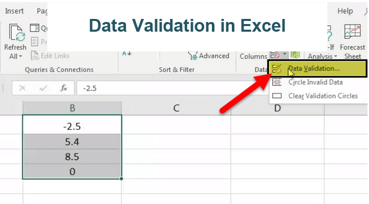
The following image shows a list of numbers in column B. We want to perform the following tasks:

Show how to create a data validation rule on the range B1:B4.
Explain the tabs of the “data validation” window.

The steps explaining the creation of a data validation rule in Excel are listed as follows:

Select the cells on which the data validation rule has to be created. So, select the range B1:B4.
Click the data validation drop-down (in the “data tools” group) from the Data tab of Excel. The same is shown in the following image.
Select “data validation” from the drop-down list.
The “data validation” window appears, as shown in the following image.
The first tab is “settings,” which contains the validation criteria. The same is shown in the succeeding image.

From the drop-down list under “allow,” one can select the data format allowed to the users. The drop-down list under “data” is used for defining the criteria.

For instance, if the input should be entered as a whole number, select the same from the drop-down list under “allow.” Once “whole number” is selected, one can choose the minimum and the maximum range between which this number is allowed to be entered.

Likewise, the desired validation criteria can be defined for the user.

Note: Refer to the topics “The Different Data Formats” and “The Different Validation Criteria” of this article for more information on adding validation criteria.
The checkbox “ignore blank” is selected by default. This selection tells Excel to ignore the blank values.
The second tab is “input message,” as shown in the succeeding image. One can enter the “title” and the “input message,” which are displayed when a validated cell is selected.

Note: An “input message” tells the user about the kind of input allowed in a validated cell. However, it is optional to add an input message. But, if one does add an input message, ensure that the checkbox of “show input message when cell is selected” is checked.
The third tab is “error alert.” In this tab, one can enter the “title” and the “error message” that are displayed on typing invalid data in the validated cell.

From the “style” drop-down, one can select any of the three options, “stop,” “warning” or “information.” These are shown in the succeeding image.

Note 1: An “error message” is a customized message which tells the user that he/she has made an error while typing data in the validated cell. However, it is optional to add an error message. If an error message is added, ensure that the checkbox of “show error alert after invalid data is entered” is checked.

Note 2: In case an error message is not added, Excel displays the default error message, which states that restrictions have been defined for the validated cell.

Note 3: For more information on the error alert styles, refer to the topic “The Different Error Alert Styles” of this article.
Once the entries in the three tabs, “settings,” “input message,” and “error alert” have been defined, click “Ok” in the “data validation” window.

The data validation excel rule is applied to the selected range B1:B4. Likewise, one can create a data validation rule by selecting either a single cell or a range of cells in Excel.

Note: For creating a data validation rule, it is mandatory to enter the validation criteria in the “settings” tab (step 5). However, it is optional to define the tabs “input message” (step 7) and “error alert” (step 8).

Data Validation in Excel Explained in Video

Example #2–Decimal Number Validation

Working on the data of example #1, we want to perform the following tasks:

Create a data validation excel rule on cell B1. In this cell, a decimal number greater than or equal to zero is allowed to be entered.
Define an input message which appears on selecting cell B1. The title should be “negative number detected” and the message should be “enter number greater than zero.”

The steps for performing the stated tasks are listed as follows:

Step 1: Select cell B1 which contains -2.5. From the Data tab of Excel, click the “data validation” drop-down. Select “data validation.”

Step 2: The “data validation” window appears, as shown in the following image. In the “settings” tab, select “decimal” under the “allow” drop-down.

Under the “data” drop-down, select “greater than or equal to.” In the box under “minimum,” enter “0” (without the double quotation marks).

data” drop-down, select “greater than or equal to

Step 3: In the “input message” tab, select the checkbox of “show input message when cell is selected.”

In the box under “title,” type “negative number detected” without the double quotation marks. In the box “input message,” type “enter number greater than zero.” This should also be written without the double quotation marks. Click “Ok.”

The data validation rule is created on cell B1. To cross-check it, select the validated cell B1. The defined input message appears, as shown in the following image.

Defined input message

The number -2.5 was already there in cell B1 before the creation of the validation rule. This number is not deleted (from cell B1) even after creating a data validation rule.

However, in future, if a number is entered in cell B1, it must conform to the newly created rule. This implies that a decimal number greater than or equal to zero can be entered in cell B1. So, negative numbers are restricted in this cell. In case this rule is not complied with, Excel will display the default error alert.

Data Formats in Data validation

While entering data in a validated cell, there are certain formats that are allowed to the user. The rule creator (who is creating the data validation rule) can pick any of these formats based on which a validation rule can be created.

In the “settings” tab of the “data validation” window, the “allow” drop-down shows the following formats:

Any value: This implies that no validation will be executed. In case a data validation rule is created and then “any value” is selected, the created validation rule is removed. However, the input message of the created validation rule can be viewed even after “any value” has been selected.
Whole number: This requires that the user should enter a whole number in the validated cell.
Decimal: This implies that the data format allowed in the validated cell is decimal numbers.
List: This implies that the format allowed is a drop-down list. So, a drop-down list consisting of pre-defined values needs to be created. This drop-down list can be created in any of the following ways:
- Supply the values directly in the box under “source.”
- Provide the reference to the range (in the “source” box), which consists of the required values.
- Enter the name of the named range (in the “source” box), which begins with an “equal to” (=) sign.
Date: This implies that the user can enter only a date in the validated cell.
Time: This implies that a time value should be entered in the validated cell.
Text Length: This helps fix the number of digits or text entered in a validated cell. For instance, the user can enter either numbers or text up to 5 digits or 5 characters respectively.
Custom: This allows one to create a formula. This formula is used to validate (restrict) the input entered by the user. For instance, a formula can be entered to ensure that a text entry ends with certain characters, the text should be in uppercase or the entry must only be numeric, etc.

The Different Validation Criteria

Excel presents different criteria for validating data. The rule creator can select any of these criteria. Based on this selection, one can set the limits within which the input is allowed.

In the “settings” tab of the “data validation” dialog box, the drop-down under “data” shows the following validating criteria:

Between: This implies that the input should be between the minimum and the maximum numbers specified.
Not between: This implies that the input should not be between the minimum and the maximum numbers specified.
Equal to: This implies that the input should be equal to the specified value. In other words, the input should be the same as the specified value.
Not equal to: This implies that the input should not be equal to the specified value. In other words, the input should be different from the specified value.
Greater than: This implies that the input should be greater than the minimum number specified.
Less than: This implies that the input should be lesser than the maximum number specified.
Greater than or equal to: This implies that the input should be greater than or equal to the minimum number specified.
Less than or equal to: This implies that the input should be lesser than or equal to the maximum number specified.

The Different Error Alert Styles

There are different error alert styles in Excel. The rule creator can select any of these styles to notify the user that an error has been made while typing data in the validated cell.

In the “error alert” tab of the “data validation” window, the drop-down under “style” presents the following options:

Stop: This stops the users from entering invalid data in the validated cell. With the “stop” style, the error alert message presents the following main options to the user:
- Retry– Clicking “retry” allows typing a new input.
- Cancel–Clicking “cancel” deletes the invalid input.

The “stop” style is the default error alert style of Excel.

Data Validation - Stop

Warning: This warns the users that an invalid input has been entered. However, it does not stop the user from entering incorrect data. With the “warning” style, the user is presented with the following main options:
- Yes–Clicking “yes” makes Excel accept the invalid input.
- No–Clicking “no” allows typing a new input.
- Cancel–Clicking “cancel” deletes the invalid input.

Warning

Information: This informs the user that the input entered is invalid. Like the “warning” style, this also does not stop the user from entering incorrect data. With the “information” style, the user is presented with the following main options:
- Ok–Clicking “Ok” makes Excel accept the invalid input.
- Cancel–Clicking “cancel” deletes the invalid input.

Information

By selecting a style, its respective icon appears in the error alert message displayed by Excel.

For instance, with the “stop” style, the cross within the red circle is shown (in the error alert message) as the user enters invalid data. Likewise, with the “warning” and “information” styles, the exclamation mark (within a yellow triangle) and the “i” sign (within a blue circle) show up respectively.

Note: Apart from the main options listed (in the preceding pointers 1, 2, and 3), Excel also displays the “help” option in all the error alert messages, irrespective of the style selected.

Purpose of Data Validation in Excel

The objectives of data validation in excel are listed as follows:

To restrict the users from entering unwanted or incorrect data values in the worksheet
To sort and study the data obtained with the help of defined criteria
To suggest the valid data format to the users through customized input messages (displayed when a validated cell is selected)

Excel Data validation is particularly helpful in the following situations:

When the number of users is large and there is a possibility of entering inputs in different formats
When the allowed entries need to be defined with a drop-down list
When an error alert (warning message) needs to be displayed on entering invalid data

The Limitations of Data Validation in Excel

The limitations of data validation in excel are listed as follows:

Data validation in excel does not prevent a user from copying an incorrect input from a non-validated cell to a validated cell. It can stop one from typing an incorrect input but not from copying the same. Hence, the purpose of data validation can become pointless if a user copies and pastes an invalid input.
Excel Data validation cannot fully protect a worksheet from invalid data entries. If a user copies an incorrect input from a non-validated cell and pastes it in a validated cell, the validation rule in the latter cell is eliminated. As a result, the validation rule is absent on the copied data.

Frequently Asked Questions

1. Define data validation in Excel.

Data validation restricts (limits) the type of input entered by a user in the worksheet. One can set the criteria for a specific cell and ensure that the input typed (in that cell) complies with it.

For instance, in cell A1, one is allowed to type only a decimal number between 1.5 and 9.5. This is a data validation rule applied to cell A1 of the worksheet.

2. How can a data validation rule be edited in Excel?

Let us say that rule X has been applied to cells A1 and D1. We want to change this to rule Y for both the mentioned cells.

The steps to edit a data validation rule are listed as follows:

a. Select any of the cells to which rule X has been applied.
b. Select “data validation” from the “data validation” drop-down (in the “data tools” group) of the Data tab.
c. In the “settings” tab of the “data validation” window, enter the new criteria as per rule Y.
d. Select the checkbox of “apply these changes to all other cells with the same settings.” This ensures that rule Y is applied to both the cells A1 and D1.
e. Click “Ok.”

The rule Y has been applied to both cells A1 and D1.

Note: The new data validation rule can be applied to all the validated cells only if they all had the same validation criteria initially. In this case, the initial validation criterion (rule X) was the same for both the validated cells (A1 and D1).

3. How can a data validation rule be removed in Excel?

The steps to remove (delete) a data validation rule are listed as follows:

a. Select the validated cell.
b. From the “data validation” drop-down (in the “data tools” group) of the Data tab, select “data validation.”
c. The “data validation” window opens. In the “settings” tab, click “clear all” appearing at the bottom left side.
d. Click “Ok.”

The validation rule will be cleared from the selected cell (selected in step a).

Note: To remove the same validation rule applied to multiple cells, select the checkbox of “apply these changes to all other cells with the same settings.” Thereafter, click “clear all” followed by “Ok.”