Table Of Contents
What Is Randomize List In Excel?
Randomize list in Excel helps users to insert a new column of random numeric values, to sort a list of any data randomly, that keeps updating whenever we calculate, refresh, or open the worksheet. We can generate random numeric values using the RAND() or RANDBETWEEN() functions that give shuffled, non-repeated, unique values within a default range 0 to 1, or within a defined range, respectively.
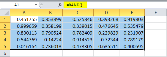
For example, enter the formula =RAND(), press “Enter” in cell A1, and drag the formula using the fill handle till cell A5.

The output is shown above. i.e., 5 random numeric values within the default range 0 to 1 are generated. We can see each value is unique and not repeated. Using this method, we can add such columns next to the required list and sort the data randomly, as we will see in the article.
Key Takeaways
- The Randomize list in Excel is a way to add a column of generated a list of random numbers in a dataset for random sorting using the related functions within a specific range.
- The RAND Excel function generates random numbers from 0 to 1, by default. However, we can generate numbers within any desired range, such as 0 to 100, 45000 to 98000, also.
- If we do not want the RAND() and the RANDBETWEEN() function generated values to recalculate when the worksheet is opened, or refreshed,
- then we can copy the generated values with the shortcut keys Ctrl + C and as paste them as cell values and not as the formula results. Therefore, we will have a set of constant values.
How To Randomize List In Excel?
We can generate an Excel Randomize List using two Excel formulas, namely:
- =RAND() function, which gives any random values to the cell. Then we can sort the list.
- =RANDBETWEEN() function offers random values to the cell from the user’s number range.
Examples
We will consider some examples to understand Randomize list in Excel.
Example #1 - Insert Random Numbers in the List by Using RAND function
We are aware that we can insert random numbers in the list from 0 to less than 1 in Excel using the RAND function. Then, using the numbers generated by the RAND function, we can sort the list of numbers randomly.
The RAND function does not have any parameters to satisfy. Therefore, we must insert the formula and close the bracket. The RAND function automatically assumes the parameter is greater than 0 and less than 1.
Let us consider an example. In the data given below, we have just entered formulas.
We have a list of products that we want to sort randomly for some confidentiality.
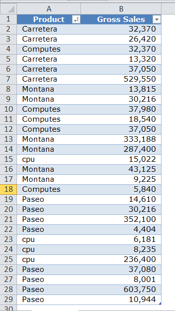
- If we try to sort the data based on the product name, it will sort either from A to Z or Z to A.
- If we try to sort the data based on gross sales, it will sort from lowest to highest or from highest to lowest.
But we want neither of them to happen. We want to sort randomly.
Below are the steps to insert random numbers in Excel: –
- Apply the RAND function immediately after the “Gross Sales” column. Then, name the new column “Helper.”

- Remember, the RAND function is volatile and keeps changing the values after every action in Excel. So, remove the formula by using the Paste Special.
- After pasting values, select the entire data range, and go to the “Data” tab.
- Under the “Data” tab, select the “Sort” option.

- Now, under the “Sort by,” select the newly inserted column, “Helper.”

- In the same window, under “Order,” select the option you want. Because we are sorting manually, we can choose any available options. We have chosen the “Smallest to Largest.”

- Click the “OK” button. It will sort the data randomly, as shown below.

Example #2 - Pick a Lottery Winner with Randomize List in Excel
If you have seen the lottery industry, they will randomly pick the winner without bias. We can also select a winner using Excel and the RAND function.
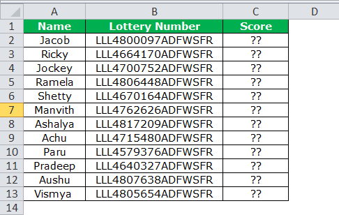
We have a few names and lottery ticket numbers given below, and we must pick a winner from this lot.

The criteria to pick a winner is to generate random numbers from 1 to 100 against each name, and whoever gets the maximum score will be declared the winner.
By using the RAND function, we will generate some numbers against each name. The problem is that the RAND function may give us all the values less than 1, so we will multiply the number 100 by the numbers generated by the RAND function.
Since the RAND function is volatile, we will remove the formula and retain only values.
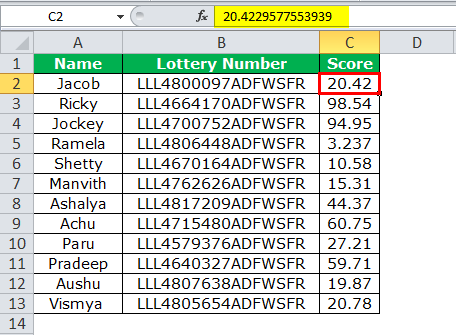
Now, we have the score ready against each name. The criteria are whoever gets the maximum score will be declared the winner. We will sort the numbers from largest to smallest as follows:
- Step 1: Select winner the data, and under the “Data” tab, select the “Sort” option.
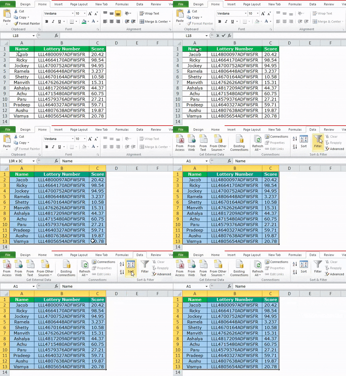
- Step 2: Under the “Sort by”, select the column “Score.”

- Step 3: Now comes the important part of the process. Under “Order,” we must select the criteria as “Largest to Smallest” so that the largest value from the list comes first.
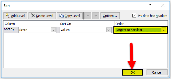
- Step 4: Click the “OK” button. It will sort the data from the largest to the smallest of the scoring column.
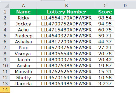
Now, we have a winner here. The winner is Ramela, who got the highest score when we applied the RAND function.
Benefits Of A Randomize List In Excel
A few benefits of using the Randomize list in Excel are as follows:
- The results in scenarios like lottery winners will be unbiased, random, and unpredictable.
- The data sharing or modifications will remain confidential, as we will see only the random numbers getting sorted, but not the other columns with important details.
- In a small or large dataset, it is impossible to memorize or remember the order of the list with its accompanying random numbers.
Important Things To Note
- Both the RAND and RANDBETWEEN are volatile functions. It will slow down the workbook considerably.
- Both functions recalculate values when there is any change that occurs in the worksheets.
- Using the RAND function, we can generate random numbers greater than 0 but less than 1.
- Do not keep volatile functions in any of the workbooks.

