Auditing Tools In Excel

Auditing tools in Excel are tools used for auditing. MS Excel is mainly used and famous for its function, formulas, and macros. But what if we are getting some issue while writing the formula, or we cannot get the desired result in a cell as we have not formulated the function correctly? That is why MS Excel provides many built-in tools for formula auditing and troubleshooting formulas.

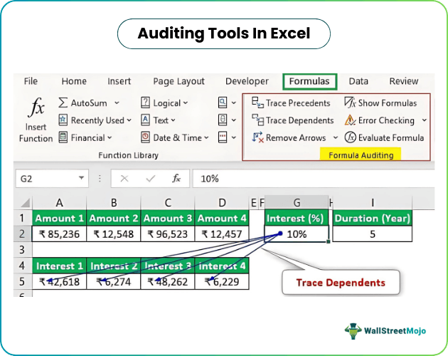
The tools which we can use for auditing and formula troubleshooting in Excel are:

1. Trace Precedents
2. Trace Dependents
3. Remove Arrows
4. Show Formulas
5. Error Checking
6. Evaluate Formula

• The auditing tools in Excel that we can use to audit and troubleshoot formulas are trace precedents, trace dependents, remove arrows, show formulas, error checking, and evaluate formulas.
• One may view the dates in number format. In addition, one can utilize the 'Show Formulas' command.
• In Microsoft Excel, one way to simplify the process of evaluating formulas is to use the "F9" shortcut on your keyboard. As a result, one can save time and enhance efficiency while working on complicated Excel spreadsheets.

We will learn about each of the above auditing tools, using some examples in Excel.

Example #1 - Trace Precedents

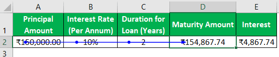
Suppose we have the following formula in the D2 cell for calculating interest for an FD account in a bank.

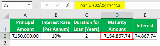
If we want to check the formula's precedents, we can press F2 to get into edit mode after selecting the required cell so that precedents cells got bordered with various colors and written in the same color and cell reference.

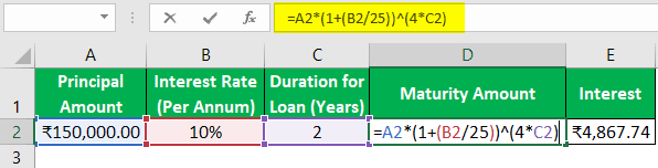
We can see that A2 is in blue color in the formula cell. Similarly, cell A2 is highlighted in blue color.

In the same way,

B2 cell has a red color.

C2 cell has a purple color.

This way is good. But we have a more convenient way to check precedents for the formula cell.

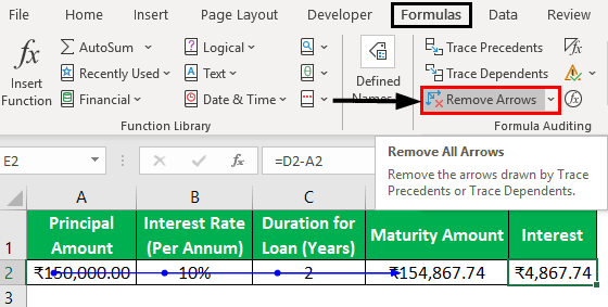
We can use the "Trace Precedents" command in the "Formula Auditing" group under the "Formulas" tab to trace precedents.

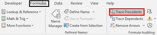
We need to select the formula cell and click on the "Trace Precedents" command. Then, you can see an arrow as shown below.

We can see that precedent cells are highlighted with blue dots.

Example #2 - Remove Arrows

We can use the "Remove Arrows" command in the "Formula Auditing" group under the "Formulas" tab to remove these arrows.

Example #3 - Trace Dependents

This command traces the cell, dependent on the selected cell.

Let us use this command using an example.

Suppose we have four amounts that we can invest in. We want to know how much interest we can earn if we invest.

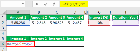
Suppose we have four amounts that we can invest in. We want to know how much interest we can earn if we invest.

We will copy the formula and paste it into the adjacent cells for amount 2, amount 3, and amount 4. One can notice that we have used an absolute cell reference for G2 and I2 cells as we do not want to change these references while copying and pasting.

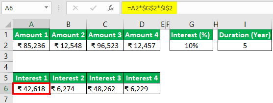
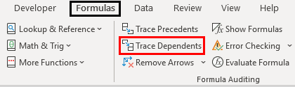
If we want to check which cells are dependent on the G2 cell, we will use the "Trace Dependents" command available in the "Formula Auditing" group under the "Formulas" tab.

Next, select the G2 cell and click on the “Trace Dependents” command.

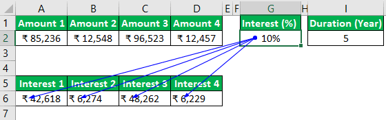
In the above image, we can see the arrow lines where arrows indicate which cells are dependent on the cells.

We will remove the arrow lines using the ‘Remove Arrows’ command.

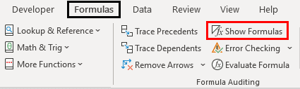
Example #4 - Show Formulas

We can use this command to display formulas written in the excel sheet. The shortcut key for this command is ‘Ctrl+~.’

Next, see the below image, where we can see the formulas in the cell.

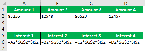
Now, we can see that we can see the formula instead of the formula results. For amounts, the currency format is not visible.

Then, press ‘Ctrl+~’ again or click on the ‘Show Formulas’ command to deactivate this mode.

Example #5 - Error Checking

This command is used to check the specified formula or function error.

See the below image where we have an error in the function applied for the result.

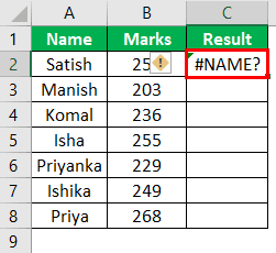
Now, we will use the “Error Checking” command to solve this error.

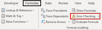
Next, select the cell where the formula or function, and then click on “Error Checking.”

Next, we will get the following dialog box “Error Checking.”

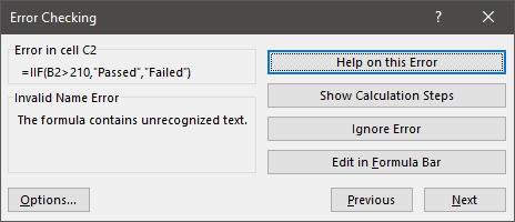
In the above dialog box, it can be seen that there is some invalid name error. Therefore, the formula contains unrecognized text.

Suppose we use the function or construct the formula for the first time. In that case, we can click on the “Help on this Error” button, which will open the help page for the function in the browser, where we can see all the related information online, understand the cause, and find all the possible solutions.

We will find the following page.

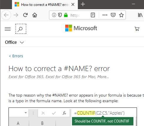
On this page, we get to know about the error that this error occurs when:

1. The formula refers to a name that has not been defined. For example, the function name or named range has not been described earlier.
2. The formula has a typo in the defined name. It means that there is some typing error.

If we have used the function earlier and know about the function, then we can click on the "Show Calculation Steps" button to check how the evaluation of the function results in an error.

• The next dialog box displays when we click on the "Show Calculation Steps" button.

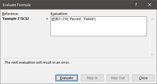
• After clicking on the "Evaluate" button, the underlined expression, i.e., "IIF," gets evaluated and gives the following information as displayed in the dialog box.

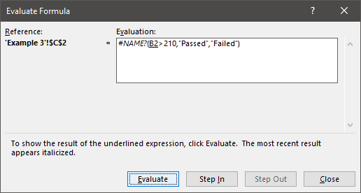
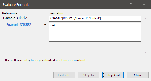
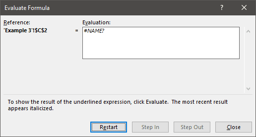
We can see that the "IIF" expression is shown as #NAME? error. The following expression or reference, i.e., B2, is underlined. If we click on the "Step In" button, we can also check the internal details and come out by pressing the "Step Out" button.

Now, we will click on the "Evaluate" button to check the result of the underlined expression. After clicking, we get the following result.

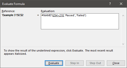
• We will get the result of the function.

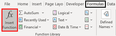
• We got an error. As a result, as we analyzed the function step by step, we learned that there was some error in "IIF." We can use the "Insert Function" command in the "Function Library" group under the "Formulas" tab.

Now, we got a similar function in the list; we need to choose the appropriate function.

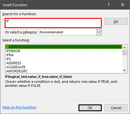
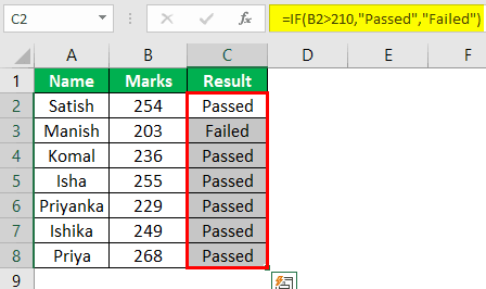
After selecting the "IF" function, we get the following dialog box with text boxes for argument, and we need to fill in all the details.

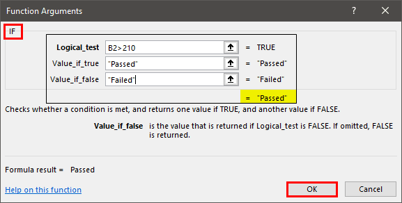
After clicking on "OK," we get the result in the cell. Next, we will copy down the function for all the students.

• The dates are also shown in the number format if we activate the ‘Show Formulas’ command.
• While evaluating the formula, we can also use "F9" as a shortcut in Excel.

This article is a guide to Auditing Tools in Excel. Here, we discuss 5 different auditing tools, including show formulas, error checking, trace precedents, etc., with some examples and a downloadable Excel template. You may learn more about Excel from the following articles: -

• Quick Analysis Tools in Excel
• PERCENTRANK in Excel
• Excel Watch Window
• Excel Structured References