Absolute Reference in Excel

A absolute reference is excel is a cell reference wherein the column and row coordinates remain fixed on copying a formula from one cell to the other. To fix the coordinates, a dollar sign ($) is placed before them. For example, $D$2 is an absolute reference that refers to cell D2. Shortcut to Absolute Reference in excel is the key F4

The purpose of making the cell reference absolute is to keep it static irrespective of whether the formula is copied to a different worksheet or workbook. By default, a cell reference in Excel is relative (like D2), implying that it changes when the formula is copied.

Apart from absolute and relative, a cell reference can also be mixed. In a mixed reference, either the column label or the row number is kept constant (like $D2 or D$2).

The shortcut to absolute reference in excel is F4. With a single keystroke, the F4 key on your keyboard allows you to add both dollar signs.

While working in Excel, it is essential to know whether a cell reference should stay absolute, relative reference or mixed. This helps one to carry out the calculations as desired.

With this article, we will focus on absolute references of Excel. Let us consider some examples to understand the working of these references in Excel.

Example #1–Multiplication Formula Using Absolute and Relative References

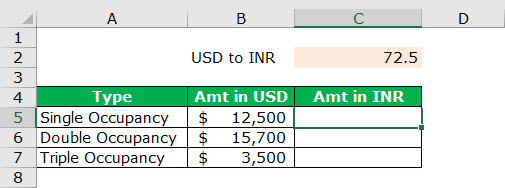
The following image shows the rates (in USD in column B) of different rooms of a hotel. We want to convert each amount from USD to INR (in column C).

Assume that 1 USD is equal to Rs. 72.5. This USD to INR conversion rate is given in cell C2. Use absolute and relative references in the multiplication excel formula. Explain the cell references used for the given task.

Explanation of the cell references: In the formulas of column C, the first cell reference is relative (B5, B6, and B7), while the second cell reference is absolute ($C$2). The reason is that on copying the formula from cell C5 to C7, we wanted the first reference to change and the second reference to stay constant.

As a result, B5 (in cell C5) changes to B6 (in cell C6) and further changes to B7 (in cell B7). However, the reference $C$2 stays the same in cells C5, C6, and C7. So, the aim is to multiply the different amounts of column B with the same conversion rate of cell C2.

Example #2–SUMIFS Formula Using Absolute and Mixed References

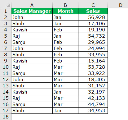
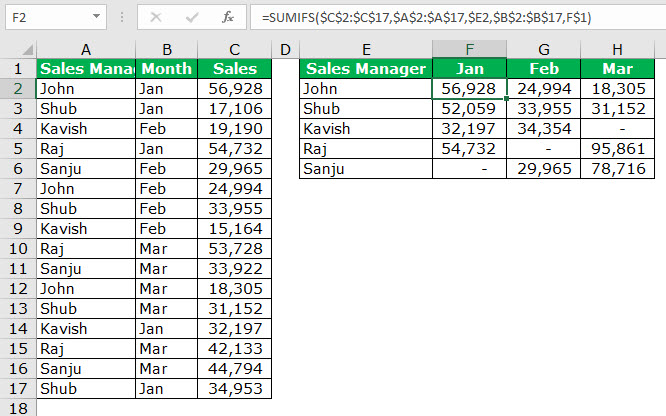
The following image shows the sales revenue generated (in $ in column C) in three months (column B) by five sales managers (in column A) of an organization. The three months are January, February, and March. The five sales managers are John, Shub, Kavish, Raj, and Sanju.

Since some sales managers have made multiple sales in a month, their names appear more than once against a single month. Sum the sales revenues generated by each manager in a particular month. Use the SUMIFS function of Excel.

Further, use the following types of cell references for the given task:

• For “sum_range,” “criteria_range1,” and “criteria_range2,” use absolute excel references.
• For “criteria1” and “criteria2,” use mixed references.

Explain the formula and the cell references used.

The steps to perform the given task by using the SUMIFS function and the stated references are listed as follows:

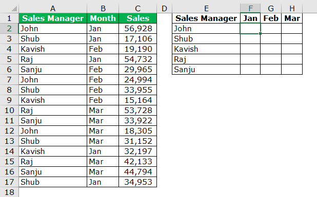
Step 1: Write the names of the five managers in the range E2:E6. Enter the names of the three months in the range F1 to H1. All these names (shown in the following image) will be used in the SUMIFS formula one at a time.

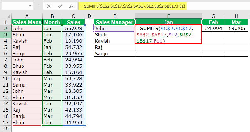
Step 2: Enter the following formula in cell F2.

“=SUMIFS($C$2:$C$17,$A$2:$A$17,$E2,$B$2:$B$17,F$1)”

This is shown in the succeeding image.

Note: Please ignore the figures of cells G2 and H2 at this step.

Step 3: Drag the formula of cell F2 horizontally (till cell H2) and vertically (till cell F6). Likewise, drag the formula of cells F3, F4, F5, and F6 horizontally till cells H3, H4, H5, and H6 respectively.

The outputs of all the SUMIFS formulas are shown in the range F2:H6 of the following image. Hence, the sales revenue generated by all the managers in the given months (January, February, and March) has been obtained.

Notice that the cells containing a hyphen (F6, G5, and H4) imply that a sale has not been made in that month by the respective manager.

Explanation of the formula and the cell references: The formula of step 1 works as follows:

1. The “sum_range” supplied to the SUMIFS function is $C$2:$C$17. The numbers of this range are summed subject to the conditions (or criteria) entered in the formula. We have used absolute cell references in the “sum_range.” This is because we do not want the references to change as the formula is copied to the remaining cells of the range F2:H6.
2. The “criteria_range1” supplied to the SUMIFS function is $A$2:$A$17. This range is evaluated for “criteria1.” We have again used absolute excel references in “criteria_range1.” The reason is that the “criteria_range1” stays the same across all the SUMIFS formulas of the range F2:H6.
3. The “criteria1” supplied to the SUMIFS function is $E2. Since cell E2 contains the name “John,” the SUMIFS function checks the range A2:A17 for this name. We have used a mixed reference ($E2) for “criteria1” because we want its column label (E) to be fixed and the row number (2) to be variable. This enables the SUMIFS function to check the range A2:A17 for the values of cells E2, E3, E4, E5, and E6. So, each cell of column E (rows 2 to 6) serves as “criteria 1” in the different SUMIFS formulas of the range F2:H6.
4. The “criteria_range2” supplied to the SUMIFS function is $B$2:$B$17. This range is evaluated for “criteria2.” We have used absolute references in this range because we want the same range (B2:B17) to be evaluated each time for “criteria2.”
5. The “criteria2” supplied to the SUMIFS function is F$1. Cell F1 contains the value “Jan.” So, the SUMIFS function checks the range B2:B17 for the value “Jan.” We have used a mixed reference (F$1) for “criteria2.” This is because we want the SUMIFS function to check the range B2:B17 for the values of cells F1, G1, and H1. Thus, the column label changes from F to G and finally to H, while the row number stays constant at 1.

The SUMIFS formula of step 1 checks for two conditions (criteria) “John” and “Jan” in the ranges A2:A17 and B2:B17 respectively. Further, those values of the range C2:C17 are summed that satisfy both these conditions. So, only the number 56,928 satisfies both these conditions. Hence, the output is 56,928.

In the same way, the SUMIFS formulas of the remaining range F2:H6 work.

Note: The SUMIFS function sums those values that satisfy multiple criteria. For the syntax of the SUMIFS function, click the hyperlink given before step 1 of this example.

The important points related to cell references of Excel are listed as follows:

• In an absolute reference in excel, both the column label and the row number are fixed by placing a dollar sign ($) before them. So, an absolute reference has an absolute column and an absolute row.
• In a relative reference, both the column label and the row number are variable. The dollar sign ($) is omitted in a relative reference. So, a relative reference has a relative column and a relative row.
• In a mixed reference, either the column label or the row number is fixed, while the other is variable. The dollar sign ($) is placed before the constant part of a mixed reference. So, a mixed reference has either a relative column and an absolute row or an absolute column and a relative row.
• The absolute references in excel do not change irrespective of an upward, downward, leftward or rightward movement of the formula containing them.
• The cell references change each time the F4 key is pressed. They change as follows:
  • Pressing the F4 key once changes the cell reference from relative to absolute (like D2 changes to $D$2).
  • Pressing the F4 key twice changes the cell reference from absolute to mixed (like $D$2 changes to D$2). The column label of the mixed reference becomes variable, while the row number stays fixed.
  • Pressing the F4 key thrice changes the cell reference from mixed to mixed again (like D$2 changes to $D2). The column label of the mixed reference becomes fixed, while the row number stays variable.
  • Pressing the F4 key four times changes the cell reference from mixed to relative again (like $D2 changes to D2).

Note: The steps to change a cell reference within a formula are listed as follows:

1. Double-click the cell containing the formula.
2. Select the cell reference to be changed.
3. Press the F4 key the required number of times.
4. Complete the formula in the usual way once the cell reference has been changed. So, press either the “Enter” or the “Ctrl+Shift+Enter” keys depending on whether it is a regular or an array formula.

To exit the Edit mode without changing the formula, press the escape (Esc) key.