Part of our Data Analysis in Excel guide
What Is Compare Two Columns In Excel For The Matches?
Compare Two Columns in Excel for the Matches means comparing the cell values from columns of a dataset to find matches, and return TRUE or FALSE accordingly.
We have several methods in Excel to compare two columns for the matches. But, of course, it depends on data structure and Excel skills too.
For example, we will apply a simple formula =A1=B1 to check if the cell values match using the “=” equal sign, where A1 and B1 are cells with similar or different values.
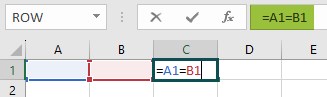
If there is a match, we will get the logical value as an output, as TRUE else FALSE.
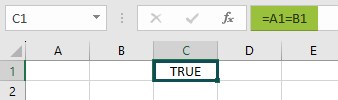
Here, the output is TRUE, as both the selected cells are empty and a match.
Key Takeaways
- Compare two columns in Excel for Matches helps us compare the cell values in 2 different columns logically to see if they are similar or different.
- The output is always one of the Boolean values, TRUE or FALSE. If wewant an alternate output, we can use the IF functions.
- We can easily match the two cells by inserting the operating symbol equal (=) sign in between the two cells.
- The EXACT function matches two cell values and considers both the cells’ case-sensitive characters.
How To Compare Two Columns In Excel For The Matches?
We can Compare Two Columns in Excel for the Matches using 2 methods, namely,
- Simple Method.
- Match Case Sensitive Values
Examples
We will consider specific examples for the above-mentioned methods.
Example #1 – Simple Method
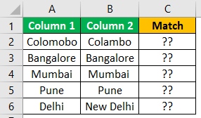
Look at the below data in two columns. We need to match the below two columns of data. But first, we must copy the above table to the worksheet in Excel.
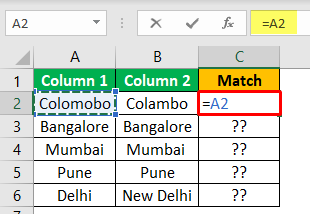
Since we are testing whether the column 1 value equals column 2, we must put the equal sign and choose the B2 cell.
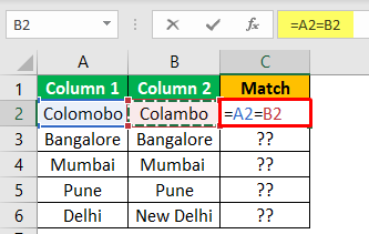
This formula checks whether the A2 cell value equals the B2 cell value. If it matches, the result will be “TRUE” or “FALSE.”
- Press the “Enter” key and apply the excel formula to other cells to get the matching result in all the cells.
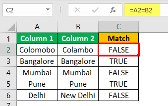
- The first result is “FALSE” because, in cell A2, we have a value of “Colomobo,” and in the B2 cell, we have a value of “Colambo”. Since these values are different, we get the matching result as “FALSE.”
- The following result is “TRUE” because, in both, the cell values are “Bangalore,” and the matching result is “TRUE.”
- The next matching result is “FALSE,” even though the cell values look similar. So, we need to dig deep to find the actual variance between these two cell values.
First, we will apply the LEN function to find the number of characters in both cells.
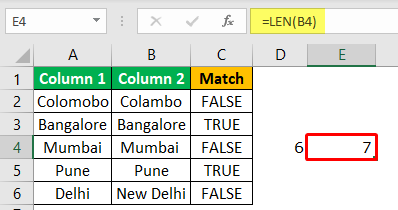
In cell A4, we have six characters. In cell B4, we have seven characters. There may be extra leading space characters, so we can use the TRIM function while applying a matching formula to deal with these scenarios. Enclose cell references in the TRIM function.
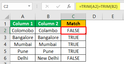
Now, look at the result in the C4 cell. It shows “TRUE” as a result, thanks to the TRIM function.
The TRIM function removes all the unwanted space characters from the selected cell reference, and space could be in three ways trailing space, leading space, and extra space.
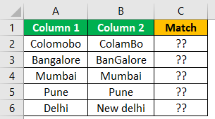
Example #2 – Match Case Sensitive Values
We can also match two column values based on a case-sensitive nature, i.e., both the cell values should be case-sensitive matches.
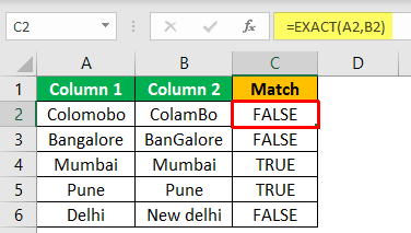
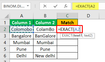
We can use Excel’s EXACT function to match two column values based on case sensitivity.
Follow the steps to match case-sensitive values.
We have modified the above data as shown below.

Then, we need to open the EXACT function. For the Text 1 argument, choose the A2 cell.

For the Text 2 argument, choose the B2 cell.

Then, close the bracket and press the Enter key to get the result.

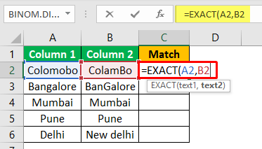

The first one is “FALSE” because both cell values differ. The second one is “FALSE,” even though the cell values are the same since the letter “G” in the second value is in the uppercase letter. Therefore, the EXACT function looks for exact values and gives the result as “FALSE” if there is any deviation in character cases.
Important Things To Note
- We can match only two cells from the same or different rows or columns at the same time using the equal sign method.
- More than two cells comparison gives an error when we use the EXACT() function.
Frequently Asked Questions (FAQs)
Can we Compare multiple columns in Excel for Matches?
Yes, we can compare multiple columns using the simple equal sign. However, using the alternate Exact function method, we can compare only two cell values, either the same or different columns.
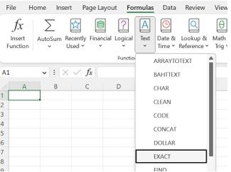
Where is the Exact function found to Compare Columns in Excel for Matches?
The Exact function is a Text function and is found using the following path,
Choose an empty cell – select the “Formulas” tab – go to the “Function Library” group – click the “Text” option drop-down – select the “Exact” function, as shown below.
The “Function Arguments” window appears. Enter the argument values in the “Text1 and Text2” fields as cell values or references, and click “OK”.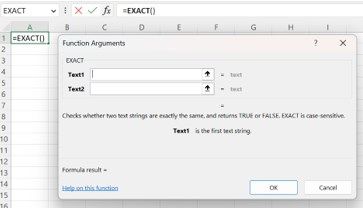
Which is the better option to compare two columns in Excel for Matches?
Although we have two methods as we just learnt to compare cell values. Each has its Pros and Cons; we can choose the desired method keeping the dataset in mind.
• The Equals method – We can compare more than 2 cell values and drag the formula. There is no limit till the Excel cell allows it.
• The Exact function method – We can compare a maximum of 2 values. However, we can drag the formula, too, for the rest of the dataset unless it is 2 column comparison.
Recommended Articles
This article is a guide to Compare Two Columns in Excel for Matches. We compare 2 values, find a match, Equals Sign(=), EXACT, examples, downloadable template. You may also look at these useful functions in Excel: –