
Table Of Contents
How to Compare Two Lists in Excel? (Top 6 Methods)
Below are the six different methods used to compare two lists of a column in Excel for matches and differences.
- Method 1: Compare Two Lists Using Equal Sign Operator
- Method 2: Match Data by Using the Row Difference Technique
- Method 3: Match Row Difference by Using the IF Condition
- Method 4: Match Data Even If There is a Row Difference
- Method 5: Highlight All the Matching Data using Conditional Formatting
- Method 6: Partial Matching Technique
Now, let us discuss each of the methods in detail with an example: -
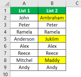
#1 - Compare Two Lists Using Equal Sign Operator
We must follow the below steps to compare the two lists.
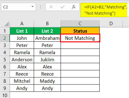
- Immediately after the two columns, we must insert a new column called “Status” in the next column.

- Now, we must put the formula in cell C2 as =A2=B2.

- This formula tests whether the cell A2 value is equal to cell B2. If both cell values are matched, we will get TRUE or FALSE results.

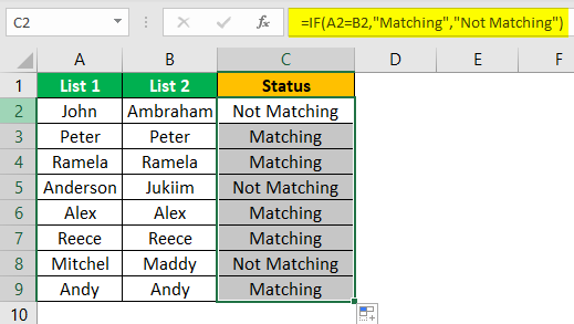
- We will drag the formula to cell C9 to determine the other values.

Wherever we have the same values in common rows, we get the result as "TRUE" or "FALSE."
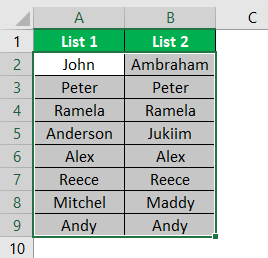
#2 - Match Data by Using Row Difference Technique
You might not have used the "Row Difference" technique at your workplace. But today, we will show you how to use this technique to match data row by row.
- Step 1: To highlight non-matching cells row by row, we must select the entire data first.
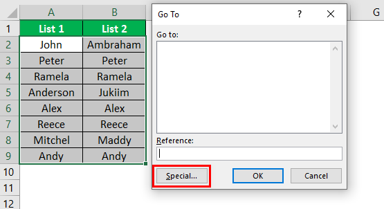
- Step 2: Now, we must press the excel shortcut key "F5" to open the "Go to Special" tool.

- Step 3: Press the "F5" key to open this window. In the "Go To" window, press the "Special" tab.
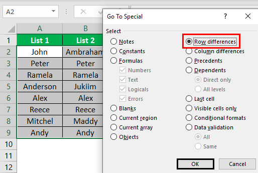
- Step 4: In the next window, we must go to the "Go To Special" and choose the "Row differences" option. Then, click on "OK."
We will get the following result.
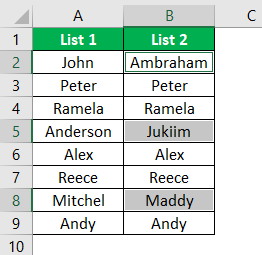
As shown in the above window, it has selected the cells wherever there is a row difference. Therefore, we must fill in some colors to highlight the row difference values.
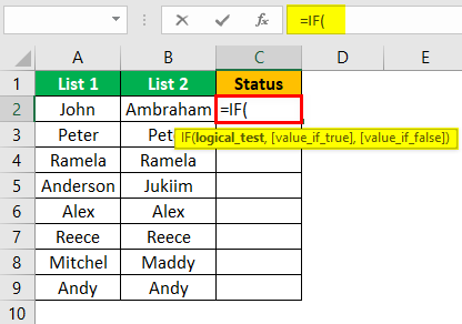
#3 - Match Row Difference by Using IF Condition
How can we leave out the IF condition when we want to match data row by row? In the first example, we have either "TRUE" or "FALSE." But what if we need a different result instead of the default results of either "TRUE or FALSE." Assume we need a result as "Matching" if there is no row difference, and the result should be "Not Matching" if there is a row difference.
- Step 1: First, we must open the IF condition in cell C2.
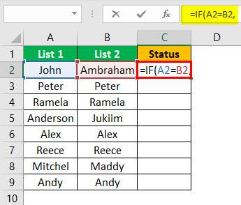
- Step 2: Then, apply the logical test as A2=B2.
- Step 3: We must enter the result criteria if the logical test is "TRUE." In this scenario, the result criteria are "Matching," If the row does not match, we need the result as "Not Matching."
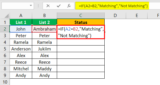
- Step 4: Next, we need to apply the formula to get the result.
- Step 5: We must drag the formula to cell C9 to determine the other values.
#4 - Match Data Even If There is a Row Difference
The matching data on the row differences method may not always work; the value may be in other cells too. So we need to use different technologies in these scenarios.
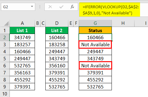
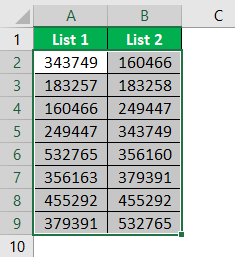
Now, look at the below data.
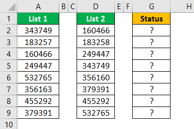
In the above image, we have two lists of numbers. We need to compare list 2 wish list 1. So let us use our favorite function VLOOKUP.
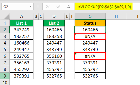
So, if the data matches, we get the number; otherwise, we get the error value as #N/A.
Showing error values does not look good. So instead of showing the error, let us replace them with the word "Not Available." For this, use the IFERROR function in Excel.
#5 - Highlight All the Matching Data
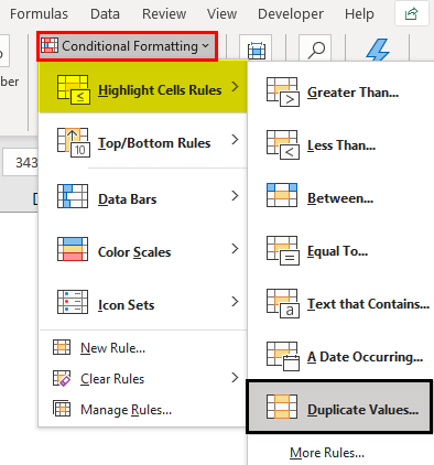
If you are not a fan of Excel formulas, do not worry. We can still match data without the formula. For example, using simple conditional formatting in Excel, we can highlight all the matching data of two lists.
- Step 1: We must first select the data.
- Step 2: Now, we must go to "Conditional Formatting" and choose "Highlight Cell Rules" >> "Duplicate Values."
- Step 3: As a result, we can see the "Duplicate Cell Values" formatting window.
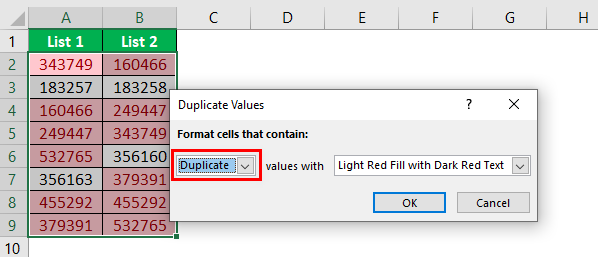
- Step 4: We can choose the different formatting colors from the drop-down list in Excel. Select the first formatting color and press the "OK" button.
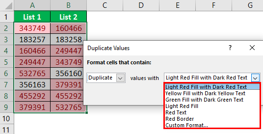
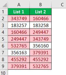
- Step 5: This will highlight all the matching data from the two lists.
- Step 6: Just in case, instead of highlighting all the matching data, if we want to highlight not matching data, then we can go to the "Duplicate Values" window and choose the option "Unique."
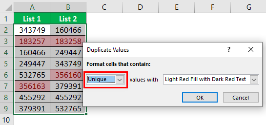
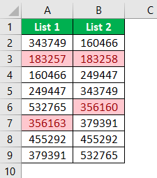
As a result, it will highlight all the non-matching values, as shown below.
#6 - Partial Matching Technique
We have seen the issue of not having full or the same data in two lists. For example, if the List 1 data has "ABC Pvt Ltd." In List 2, we have "ABC" only. In these cases, all our default formulas and tools are not recognized. Therefore, we need to employ the special character asterisk (*) to match partial values in these cases.
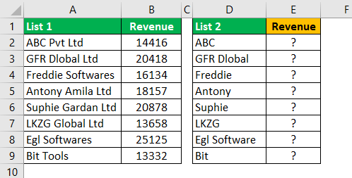
In List 1, we have the company name and revenue details. In List 2, we have company names but not exact values as in List 1. It is a tricky situation that we all have faced at our workplace.
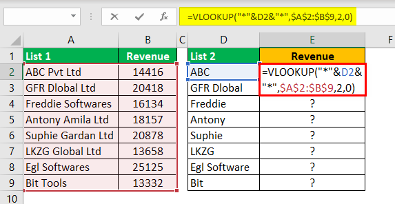
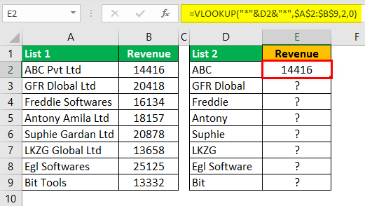
In such cases, still, we can match data by using a special character asterisk (*).
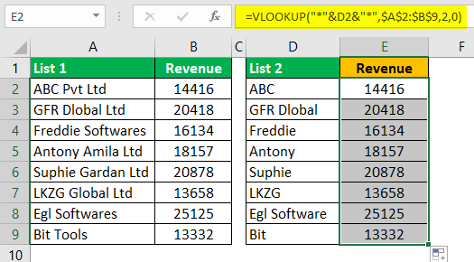
We get the following result.
We will drag the formula to cell E9 to determine the other values.
The wildcard character asterisk (*) was used to represent any number of characters so that it will match the full character for the word "ABC" as "ABC Pvt Ltd."
Things to Remember
- The use of the above techniques for comparing two lists in Excel upon the data structure.
- If the data is not organized, row-by-row matching is not the best suited.
- VLOOKUP is the often-used formula to match values.
