
Table Of Contents
Different Methods to Match Data in Excel
There are various methods to match data in Excel. For example, suppose we want to compare the data in the same column, e.g., check for duplicity. In that case, we can use "Conditional Formatting" from the "Home" tab. On the other hand, if we want to match the data in two or more different columns, we can use conditional functions like the IF function.
- Method #1 - Using Vlookup Function
- Method #2 - Using Index + Match Function
- Method #3 - Create Your Own Lookup Value
Now, let us discuss each of the methods in detail.
#1 - Match Data Using VLOOKUP Function
The VLOOKUP function is not only used to get the required information from the data table. It can also be used as a reconciliation tool. When reconciling or matching the data, the VLOOKUP formula leads the table.
- For example, look at the below table.

- We have two data tables here. The first is Data 1. The second is Data 2.
Now, we need to reconcile whether the data in the two tables match. The first way of comparing the data is the SUM function in excel to two tables to get the total sales.
Data 1 - Table
Data 2 - Table
- We have applied the SUM function for the table’s Sale Amount column. In the beginning, we have got the difference in values. The Data 1 table shows the total sales of 2,16,214, and the Data 2 table shows 2,10,214.
Now, we need to examine this in detail. So, let us apply the VLOOKUP function for each date.
- Select the table array as Data 1 range.

- We need the data from the second column, and the range of LOOKUP is FALSE, i.e., exact match.

- The output is given below:

- First, we must deduct the original value from the next cell's arrival value.

- After deducting, we get the result as zero.

- We must copy and paste the formula to all the cells to get the variance values.

- In cells G6 and G12, we got the differences.

In Data 1, we have 12,104 for 04-Mar-2019. However, in Data 2, we have 15,104 for the same date, so there is a difference of 3,000.
Similarly, for 18-Mar-2019 in Data 1, we have 19,351. In Data 2, we have 10,351, so the difference is 9,000.
#2 - Match Data Using INDEX + MATCH Function
For the same data, we can use the INDEX + MATCH function. We can use this as an alternative to the VLOOKUP function.
The INDEX function is used to get the value from the selected column based on the row number provided. We need to use the MATCH function based on the LOOKUP value to give the row number.
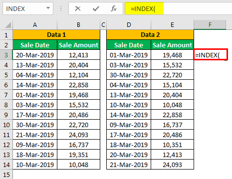
We must Open INDEX function in the F3 cell.
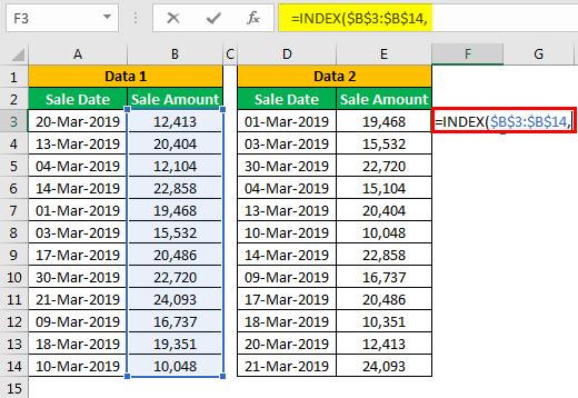
Then, select the array as a result column range, B2 to B14.
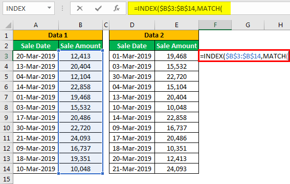
Open the MATCH function as the next argument to get the row number.
Select the LOOKUP value as a D3 cell.

Next, select the lookup array as the "Sales Date" column in Data 1.
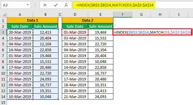
In the match type, select "0 – Exact Match."
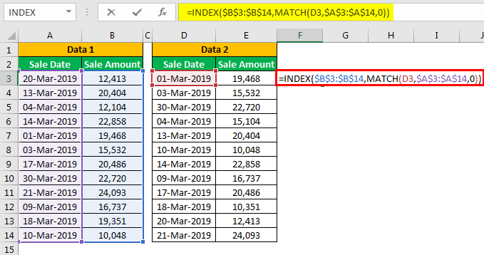
Now, close two brackets and press the "Enter" key to get the result.
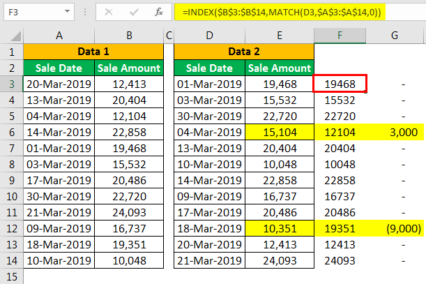
It also gives the same result as VLOOKUP. Since we have used the same data, we got the numbers as it is.
#3 - Create Your Lookup Value
Now, we have seen how to match data using Excel functions. Now, we will see the different scenarios in real-time. For this example, look at the below data.
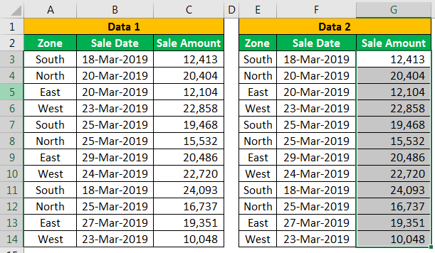
As shown above, we have zone-wise and date-wise sales data in the above data. Therefore, we need to perform the data matching process again. But, first, let us apply the VLOOKUP function as per the previous example.
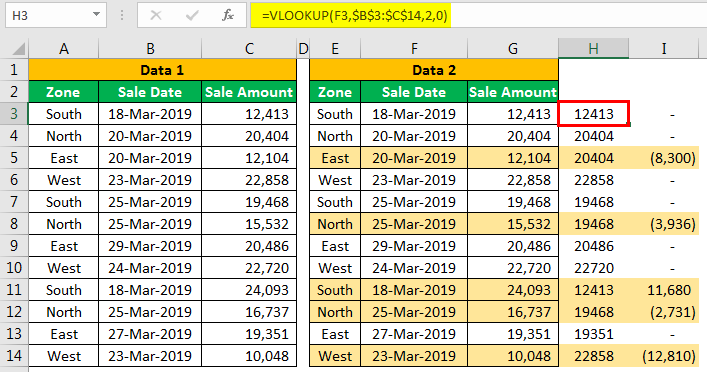
We got many variances. Let us examine each case by case.
In cell I5, we got a variance of 8,300. Let us look at the main table.
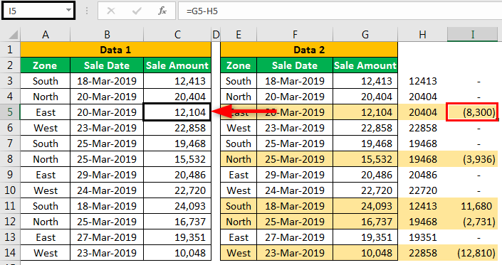
Even though the main table value is 12,104, we got the value of 20,404 from the VLOOKUP function. That is because VLOOKUP can return the first found LOOKUP value.
In this case, our LOOKUP value is a date of 20-Mar-2019. In the above cell for the "North" zone for the same date, we have a value of 20,404, so VLOOKUP has returned this value for the "East" zone.
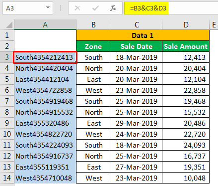
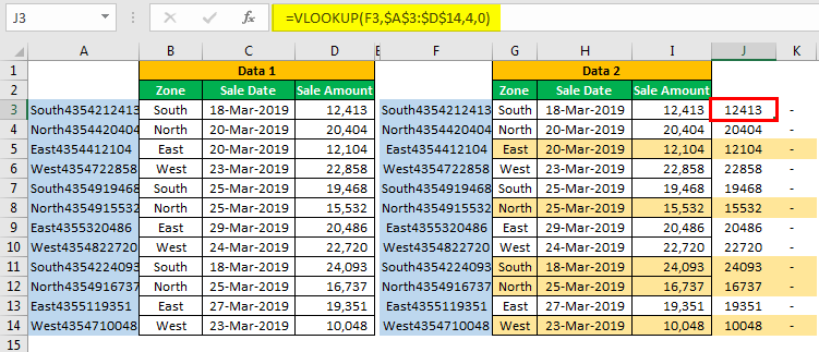
To overcome this issue, we need to create unique LOOKUP values. For example, combine Zone, Date, and Sales Amount in Data 1 and Data 2.
Data 1 - Table
Data 2 - Table
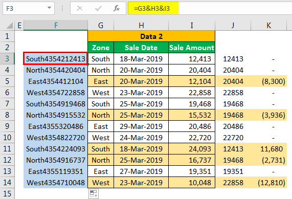
We have created unique values for each zone with the combined value of "Zone," "Sale Date," and "Sale Amount."
Using these unique values, let us apply the VLOOKUP function.
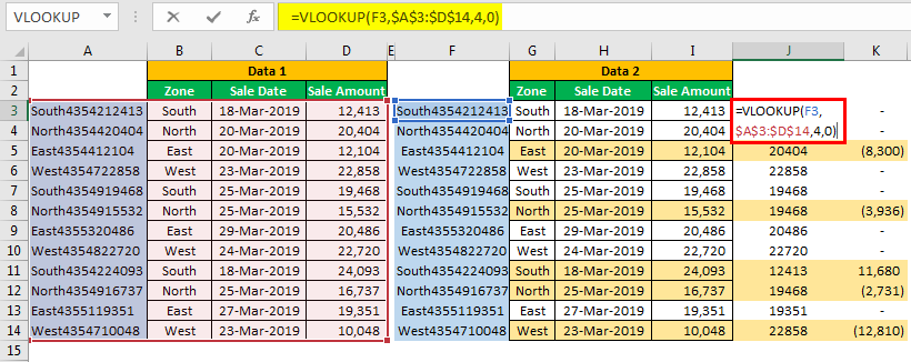
Apply the formula to all the cells. We will get the variance of zero in all the cells.
Like this, by using Excel functions, we can match the data and find the variances. First, however, we need to look at the duplicates in the LOOKUP value for accurate reconciliation before applying the formula. The above example is the best illustration of duplicate values in the LOOKUP value. We need to create our unique LOOKUP values in such scenarios and arrive at the result.
