Excel Reverse Order

The reverse order in Excel is flipping the data where the bottom value comes on top, and the top value goes to the bottom.

For example, look at the below image.

As we can see, the bottom value is at the top in the reverse order, and the same goes for the top value. So, how we reverse the order of data in Excel is the question now.

In Excel, we can sort by following several methods. Here, we will show you all the possible ways to reverse the order in Excel.

Method #1 - Simple Sort Method

You must already wonder whether it is possible to reverse the data by just using a sort option. Unfortunately, we cannot reverse just by sorting the data, but we can do this with some helper columns.

We must follow the below-given steps to reverse the order of data rows in Excel.

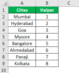
1. We must first consider the below data for this example.

   
   

2. Next, we must create a Helper column and insert serial numbers.

   
   

3. Now, select the entire data and open the sort option by pressing ALT + D + S.

   
   

4. Under Sort by, choose Helper.

   
   

5. Then, under Order, choose Largest to Smallest.

   
   

6. Now click on OK, and it will reverse our data.

   
   

Method #2 - Using Excel Formula

We can also reverse the order by using formulas. So, even though we do not have any built-in function to do this, we can use other formulas to reverse the order.

To make the reverse order of data, we can use two formulas: INDEX and ROWS. The INDEX Function can fetch the result from the mentioned row number of the selected range. The ROWS function in excel can give the count of several selected rows.

Step 1 - First, we must consider the below data for this example.

Step 2 - Then, we must open the INDEX function first.

Step 3 - For "Array," we must select the city names from A2: A9 and make it an absolute reference by pressing the "F4" key.

Step 4 - To insert RowNum, we must open the ROWS function inside the INDEX function.

Step 5 - For the ROWS function, we must select the same range of cells as we have selected for the INDEX function. But this time, it only makes the last cell an absolute reference.

Step 6 - Now, close the bracket and press the "Enter" key to get the result.

Step 7 - Drag the formula to get the full result.

Method #3 - Reverse Order by Using VBA Coding

Reversing the order of excel data is also possible by using VBA Coding. If you have good knowledge of VBA, then below is your code.

Code:

Sub Reverse_Order()    Dim k As Long    Dim LR As Long    LR = Cells(Rows.Count, 1).End(xlUp).Row    For k = 2 To LR        Cells(k, 2).Value = Cells(LR, 1).Value        LR = LR - 1    Next k End Sub

We need to copy this code to the module.

Now, run the code to get the reverse order list in the Excel worksheet.

Let us explain how this code works. First, we have declared two variables, "k" & "LR," as a "LONG" data type.

Dim k As Long Dim LR As Long

“k” is for looping through cells, and “LR” is to find the last used row in the worksheet.

Next, we have used the last used row technique to find the last value in the string.

LR = Cells(Rows.Count, 1).End(xlUp).Row

Next, we have employed FOR NEXT loop-to-loop through the cells to reverse the order.

For k = 2 To LR    Cells(k, 2).Value = Cells(LR, 1).Value    LR = LR - 1 Next k

So when we run this code, we get the following result.

• There is no built-in function or tool available in Excel to reverse the order.
• A combination of INDEX + ROWS will reverse the order.
• The "Sort" option is better and easier to sort from all the available techniques.
• To understand VBA code, we need to know VBA macros.