Sum by Color in Excel

Last Updated :

21 Aug, 2024

Blog Author :

Edited by :

Reviewed by :

Table Of Contents

What Is Sum By Color In Excel?

Sum By Color in Excel helps us identify the cell values with the same color formatting, then calculate the total sum of only those cell values in a given dataset excluding the values of the other cells that do not satisfy the given criteria.

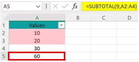
For example, in the given dataset, we have applied conditional formatting to highlight cell values less than 30. We can see in the image below that cells A2 and A3 are highlighted. In cell A5, enter the formula =SUBTOTAL(9,A2:A4), and press “Enter”.

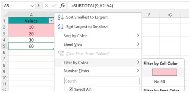
We get the total as 60. Now, Apply data filter, and filter by color, as shown below.

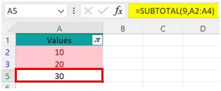
The output is the SUM of cells A2 and A3, i.e., 30, as only those cells are colored, and satisfy the criteria.

What Is Sum By Color In Excel?

The Sum By Color in Excel is a feature where we use the Conditional Formatting or Manual way to highlight specific cells. Then, we find the sum of only the highlighted cells with a specific color, ignoring the remaining values, in other words, only the sum of the cells that satisfy the condition of cell values with the same color.
While using the approach by SUBTOTAL formula, this functionality allows the users to filter for only one color at a time. Moreover, we can utilize this functionality to add only one column of values by filtering colors if there is more than one column with different colors by rows in the various columns.
The GET.CELL formula, combined with the SUMIF approach, eliminates this limitation, as we could use this functionality to summarize by colors for multiple color codes in the cell background.

Download Template

This article must help understand Sum By Color in Excel with its formulas and examples. You can download the template here to use it instantly.

How To Sum By Color In Excel? (2 Useful Methods)

We can perform the Excel Sum By Colors using 2 methods, namely:

Sum By Color using Subtotal Function – Here, we use the SUBTOTAL formula in excel and filter by color function.
Sum By Color using Get.Cell Function – It is done by Applying GET.CELL formula by defining the name in the formula tab and applying the SUMIF formula in excel to summarize the values by color codes.

Let us discuss each of them in detail with specific examples.

#1 – Sum By Color using SUBTOTAL Function

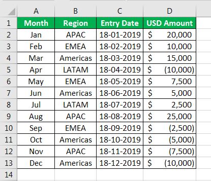
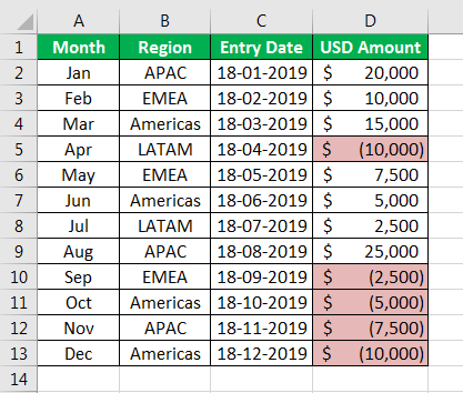
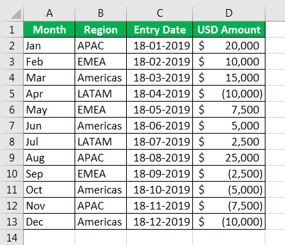
To understand the approach for calculating the sum of values by background colors, let us consider the below data table, which provides details of amounts in US$ by region and month.

The steps to apply the SUBTOTAL function to perform Sum By Color are as follows:

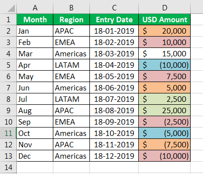
Suppose we would like to highlight those cells that are negative in values for indication purposes that can be achieved by either applying conditional formatting or manually highlighting the cells, as shown below.
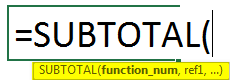
To achieve the sum of cells colored in Excel, enter the formula for SUBTOTAL below the data table. The syntax for the SUBTOTAL formula is shown below.

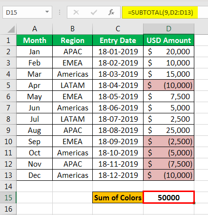
The formula that is entered to calculate the summation is =SUBTOTAL(9,D2:D13)
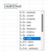
Here, the number 9 in the function_num argument refers to sum functionality, and the reference argument is given as the range of cells to be computed, as shown below.
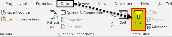
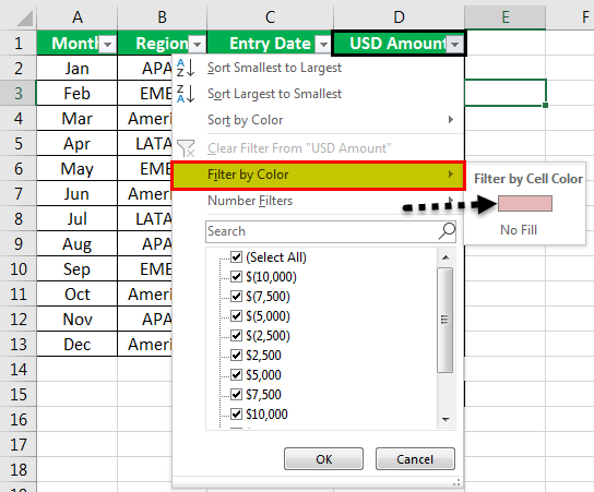
As the above screenshot shows, a “USD Amount” summation has been calculated to compute the amounts highlighted in a light red background. Next, apply the filter to the data table by going to the “Data” tab and selecting a filter.
Select filter by color and choose the light red cell color under “Filter by Color.” Below is the screenshot to better describe the filter.
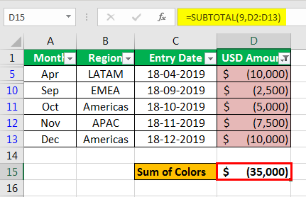
Once the Excel filter has been applied, it will filter the data table for only light red background cells. The subtotal formula used at the bottom of the data table would display the summation of the colored cells, which are filtered as shown below.

As shown in the above screenshot, the computation of the colored cell is achieved in cell E17, subtotal formula.

#2 – Sum By Color using Get.Cell Function

The second approach is explained to arrive at the sum of the color cells in Excel, as discussed in the below example. Consider the data table to understand the methodology better.

The steps to apply the GET.CELL function to perform Sum By Color are as follows:

Step 1: Now, let us highlight the list of cells in the “USD Amount” column, which we are willing to arrive at the desired sum of colored cells, as shown below.

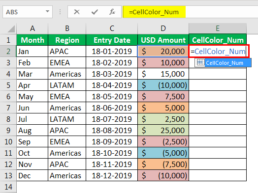
Step 2: As we can see in the above screenshot, unlike in the first example here, we have multiple colors. Therefore, we will be using the formula =GET.CELL by defining it within the name box and not directly using it in excel.
Step 3: Now, once the dialog box for the “Define Name” pops up, enter the name and the formula forgetting. CELL in “Refer to,” as shown in the below screenshot.

As seen in the above screenshot, the name entered for the function is “CellColor_Num,” and the formula =GET.CELL(38,‘Example 2’!$D2) is to be entered in ‘Refers to’. In the formula, 38 is the cell code, and D2 refers to the reference cell. Now, click “OK.”

Step 4: Now, enter the function name “CellColor” in the cell beside the color-coded cell, which was defined in the dialog box, as explained in step 3.

As seen in the above screenshot, the function “CellColor” is entered, which returns the color code for the background cell color.

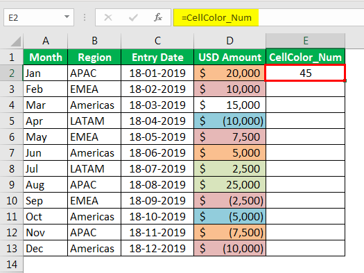
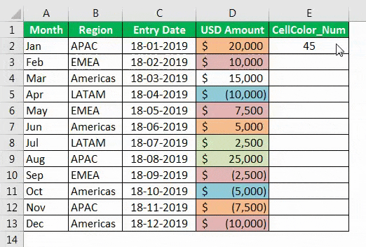
Similarly, the formula is dragged for the entire column.

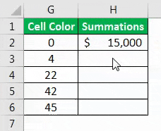
Step 5: Now, to arrive at the sum of the values by colors in Excel, we will enter the SUMIF formula. The syntax for the SUMIF formula is as follows,

As can be seen from the above screenshot, the following arguments are entered into the SUMIF formula:

The range argument is entered for cell range E2: E13.
The criteria are entered as G2, whose summarized values are needed to be retrieved.
The range of cells is entered to be D2: D13.

The SUMIF formula is dragged down for all the color code numbers for which values will be added together.

Benefits Of Sum By Color In Excel

A few benefits of Sum By Color in Excel are as follows:

We can filter the required cells and find some of the mathematical results, such as SUM, AVERAGE, MAX, MIN, COUNT, etc…
Even when the blank or empty cells are there in the dataset, we will get accurate results when we apply Conditional Formatting to find the Sum By Color.

Important Things To Note

The SUBTOTAL may only show the correct result for one filter by color to a specific column.
When using the SUBTOTAL, make sure to select 9 as an argument, as it is the number that represents SUM, as shown below.

Frequently Asked Questions

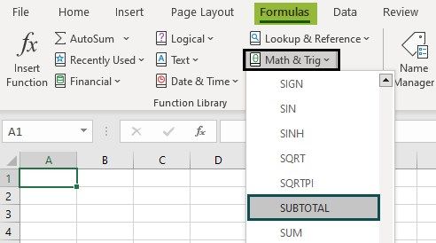
1. Where is the SUBTOTAL function in Excel found?

The SUBTOTAL function in Excel is inserted as follows:
First, choose an empty cell - select the “Formulas” tab - go to the “Function Library” group - click the “Math & Trig” option drop-down - select the “SUBTOTAL” function, as shown below.

Sum by color FAQ 1

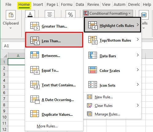
2. How can we use the Conditional Formatting in Excel to highlight cells?

We can use the Conditional Formatting in Excel as follows:
First, choose the cells or the cell range - select the “Home” tab - go to the “Styles” group - click the “Conditional Formatting” option drop-down - click the “Highlight Cell Rules” option right-arrow - select the options as per the highlight requirement, as shown below.

Sum by color FAQ 2

3. Where is the SUMIF function in Excel found?

The SUMIF function in Excel is inserted as follows:
First, choose an empty cell - select the “Formulas” tab - go to the “Function Library” group - click the “Math & Trig” option drop-down - select the “SUMIF” function, as shown below.

Sum by color FAQ 3

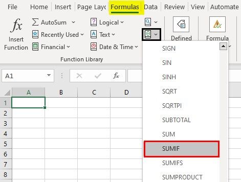
We can follow the same method to insert the “SUM” and the “SUMIFS” function, as the functions are found just above and below the “SUMIF” function, respectively.