Sort by Color in Excel

Last Updated :

Blog Author :

Edited by :

Reviewed by :

Table Of Contents

How to Sort by Color in Excel? (with Examples)

When a column or a data range in Excel is formatted with colors either by using conditional formatting or manually when we use the filter on the data, Excel provides us with an option to sort the data by color. There is also an option for advanced sorting where the user can enter different shade levels for sorting.

How to Sort by Color in Excel? (with Examples)

Example #1 - Column Sort

Recently we received a database from the Human Resources department. These include employee names and the designations in the company.

The problem is they did not mention designation against each employee. Rather, they highlighted all the executives in one color, juniors in one color, and so on. And they asked my help to sort all executives on one side, juniors on one side, and seniors on one side.

Those days we were not prolific users of the sort by color option. However, thanks to my seniors for letting me know about the sort by color in Excel early on in my career. So, even though we did not use it to the full extent, we knew there was an option called Sort by color in Excel.

Below is the data we have received from the HR department.

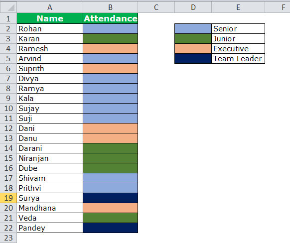
Looking at the outset, we can understand light blue represents Senior, light green represents Junior, orange represents Executive, and dark blue represents Team Leaders.

Below are the steps used for color sorting in Excel:

First, select the entire data table from A1 to B22.
Now, go to the "Data" tab (ribbon) and select "Sort." (You can press "ALT + D + S").
Once we click on "Sort," it will open up the below dialog box.

Once a small check, we need to ensure the “My data has headers” checkbox is ticked.
In “Sort by,” select the column we need to sort. In this example, we need to sort the second column, "Designation."
After this, we need to go to the "Sort On" option. Under this, select cell color.
When you select a cell color, it will enable one more option called "Order." It is simply in what order your colors should come on top. Select the color according to your wish. We have selected dark blue to go on top.
Click the "OK" button. It will sort the data based on the color of the cell. We need to notice that it will only sort the required color. All the other colored cells remain unchanged.

Note: To sort the same colors together, we need to sort four times here. Each time we need to select each color one at a time.

Example #2 - Sort By Font Colour in Excel

We can sort the data based on cell color. Similarly, we can sort the data based on the Font Color too.

Look at the below data. We have the product list region-wise. Each region’s name of the font is colored differently. We need to sort the data based on the font color.

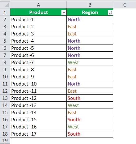
Step 1: Select the data from A1 to B18.

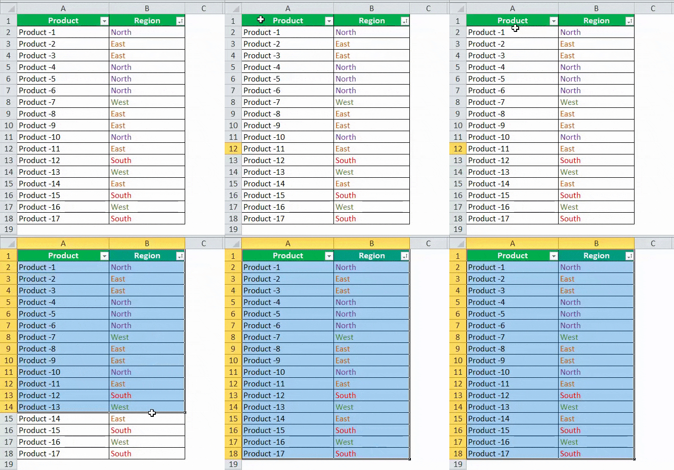
Step 2: Open the "Sort by" pressing "ALT + D + S."

Step 3: Select the column we want to sort. In this case, we have selected the "Region" column.

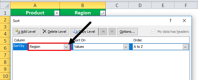
Step 4: Under the "Sort On" option, select the option "Font Color."

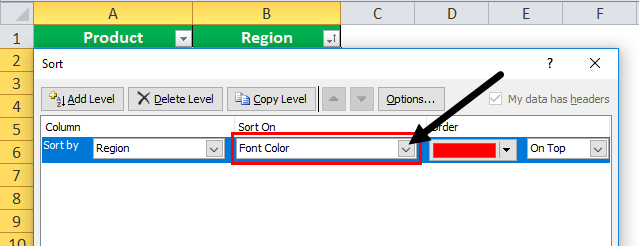
Step 5: You can choose the priority of your color under the "Order" section. We have selected "Green'' to come on top.

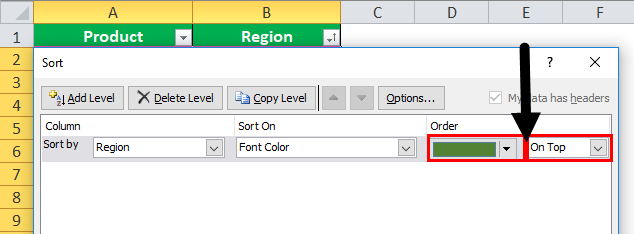
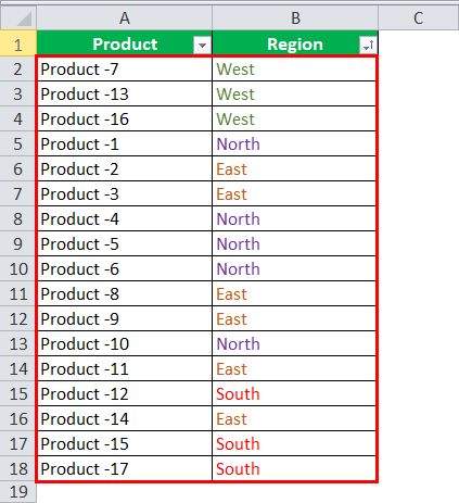
Step 6: Press the "OK" button. All the green-colored fonts will come on top, but all the other font colors remain the same.

Things to Remember

It will sort only the selected color, and all the other colored cells and fonts remain constant.
It is important to select the "My data has headers" option to avoid sorting the data headers.
We can sort one color at a time.
We can sort based on cell icons as well.
We can use a particular color to come to the top or bottom.
It is better to sort by alphabet or numbers because it will sort all the groups on one side.