Inverse Matrix in Excel

An inverse matrix is the reciprocal of a square matrix that is a non-singular matrix or invertible matrix (determinant is not equal to zero). It is hard to determine the inverse for a singular matrix. The inverse matrix in Excel has an equal number of rows and columns to the original matrix.

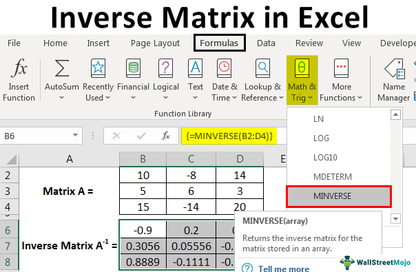
One interesting thing about the inverse matrix is that multiplying it with the original matrix will get the identity matrix with all diagonal values equal to one. That is because inverse matrices are applied in linear algebra in solving the equations. Different methods are available to determine the inverse of a matrix, including manual calculation and automated calculation. The automated analysis involves the use of Excel functions. In Excel, the matrix inverse calculation process is simplified by applying an inbuilt function of MINVERSE in excel.

Excel MINVERSE function helps return the array or matrix inverse. The input matrix must be a square matrix with all numeric values with an equal number of columns and rows in size. The INVERSE matrix will have the same dimensions as the input matrix.

Purpose: This function aims to find out the inverse of a given array.

Return value: This function returns the inverse matrix with equal dimensions.

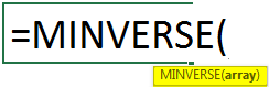
Syntax: The syntax of the MINVERSE function is

Array: The array should consist of only positive or negative numerical values.

The INVERSE function is used in two ways in Excel, including typing manually and inserting from the Math and Trig functions under the “Formula” tab.

The inverse matrix in Excel is used for various purposes. Those include:

• System of linear equations are solved in Excel using the inverse matrix
• Inverse matrices are used in non-linear equations, linear programming in excel, and finding the integer solutions to system equations.
• Inverse matrices have applications in data analysis, especially in the least square regression to determine the various statistical parameters and values of variances and covariances.
• Inverse matrices are used for resolving problems associated with the input and output analysis in economics and business.

Example#1

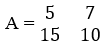
Determining the inverse of a 2×2 square matrix in Excel

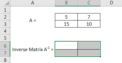
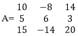
For this example, consider the following matrix A.

Follow the below steps to create a Matrix in Excel.

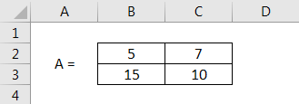
1. Enter the matrix A into the Excel sheet, as shown in the below mentioned figure.

   
   
   The range of the matrix is B2: C3.

2. Select the range of cells to position the inverse matrix A-1 on the same sheet.

   
   

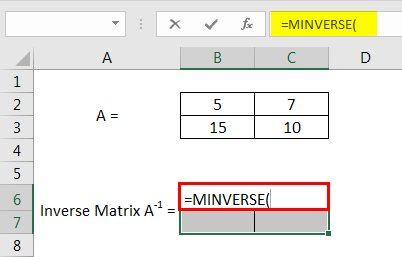
3. After selecting the required cells, we must insert the MINVERSE function formula into the formula bar. It needs to be ensured that the formula is entered while the cells are still selected.

   
   

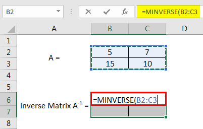
4. Then, enter the array or matrix range, as shown in the screenshot.

   
   

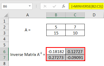
5. After entering the formula, we must press the Enter key in combination with the CTRL and SHIFT keys to convert the normal formula to an array formula to produce all elements of the inverse matrix at a time. The formula will be changed as {=MINVERSE (B2:C3)}

   
   

6. The resultant inverse matrix is produced as:

   
   
   Here, we can observe that the size of the input matrix and the inverse matrix is the same as 2×2.

Example #2

Determining the inverse of a 3×3 square matrix in Excel

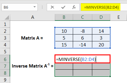
For this example, consider the following matrix A.

Step 1: We must first insert matrix A into the Excel sheet, as shown in the figure below.

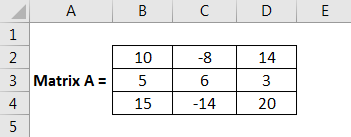
The range of Matrix A is B2: D4.

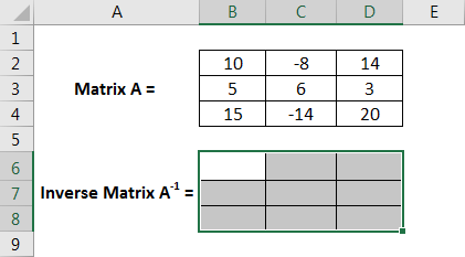
Step 2: Select the range of cells to position the inverse matrix A-1 on the same sheet.

Step 3: After selecting the required cells, enter the MINVERSE function formula into the formula bar. It needs to be ensured that the formula is entered while the cells are still selected.

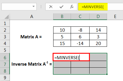
Step 4: Enter the range of the array or matrix, as shown in the screenshot.

Step 5: After entering the formula, press the "ENTER" key in combination with the "CTRL" and "SHIFT" keys to convert the normal formula to an array formula to produce all elements of the inverse matrix at a time. The formula will be changed as: {=MINVERSE (B2: D4)}

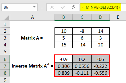
Step 6: The resultant inverse matrix is produced as:

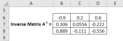
Here, we can observe that the size of the input matrix and the inverse matrix is the same as 3×3.

Example#3

Determining the inverse of the Identity matrix

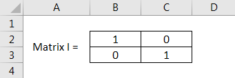
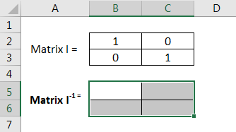
Consider the 2×2 identity matrix for this example.

Step 1: Enter the Matrix I into the Excel sheet.

Step 2: Select the range of cells to position the inverse Matrix I^-1 on the same sheet.

Step 3: After selecting the required cells, we must insert the MINVERSE function formula into the formula bar.

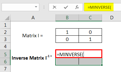
Step 4: Enter the range of the array or matrix, as shown in the screenshot.

Step 5: Press the ENTER key in combination with CTRL and SHIFT keys to convert the normal formula to an array formula. The formula will be changed as:  {=MINVERSE (B2:C3)}

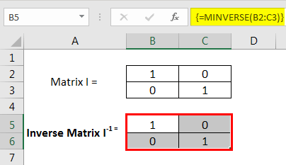
Step 6: The resultant inverse matrix is produced as:

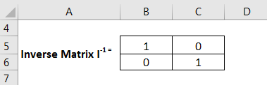
From this, it is observed that the inverse of an identity matrix and identity matrix are the same.

• While using the MINVERSE function in Excel, if the matrix contains non-numerical values, empty cells, and a different number of columns and rows, it may result in a #Value! Error.
• #NUM error shown in the provided matrix is a singular matrix.
• #N/A error displayed in the cells of the resulting inverse matrix is out of range. The MINVERSE function results in the #N/A error in extra cells selected.
• The MINVERSE function must be entered as the array formula in excel into the spreadsheet.