Excel MAXIFS

Last Updated :

Blog Author :

Edited by :

Reviewed by :

Table Of Contents

MAXIFS Function in Excel

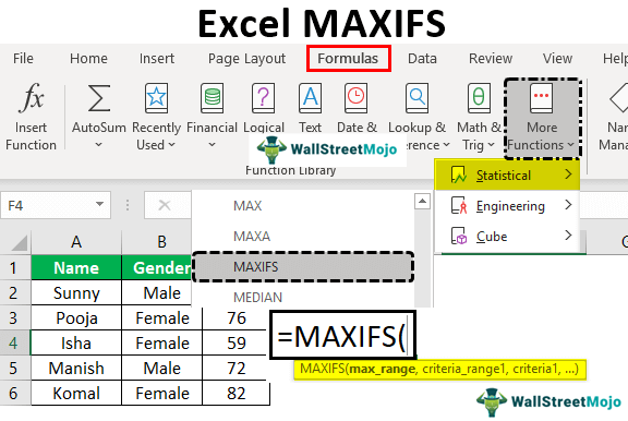
The MAXIFS function of Excel is used to get the maximum values based on various criteria. Sometimes, we have to analyze the data based on criteria. For example, we can use MAXIFS with criteria based on dates, numbers, text, and other conditions.

For example, finding out maximum marks for girls and boys separately for a class is one of the situations where we can use this function.

We can use all types of logical operators like >,<,>=,<=,<>,=, and wildcards like *,? for partial matching. For example, the condition “B? e” will match all cells containing a text string beginning with “A” and ending in “e,” and there should be only one character in between.

The condition “H*e” will match all cells containing a text string beginning with “H” and ending with “e” with multiple characters in between.

MAXIFS Function in Excel

Syntax

The formula for this function is:

The MAXIFS function returns the maximum value from a range based on multiple criteria to check in multiple ranges.

Arguments Explanation

Max Range: This is the range from where we need to find the maximum value.
Range 1: This is the range from which we will compare the values with the criteria to get the maximum value.
Criteria 1: This is the argument for the condition to specify.
Range 2: This is another range in which we will compare the values with the criteria to get the maximum value. In this way, we can provide 126 pairs of range/criteria.
Criteria 2: This is the argument for the second condition to specify.

How to Use MAXIFS Function in Excel?

Let us understand the MAXIFS function with some examples in Excel.

Example #1

Suppose we have the following data of students of a class where we have marks scored by students with their gender details.

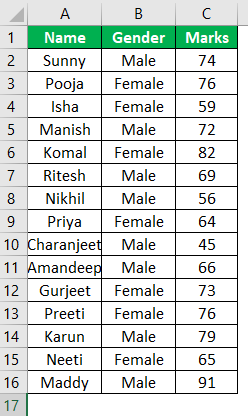
We need to find the maximum marks for females and males separately for awarding students.

To find that, we must follow the below steps:

We have created the following format for displaying maximum marks.

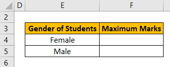
To get the maximum marks for female and male students, we will apply the MAXIFS formula.

We will refer to the cells where marks are written for the first argument as we know the syntax.

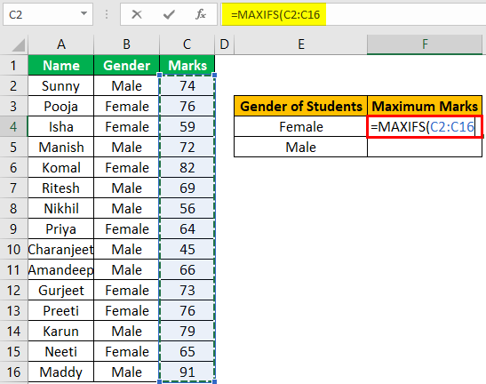
We need to select the range for the second argument where we need to check the criteria.

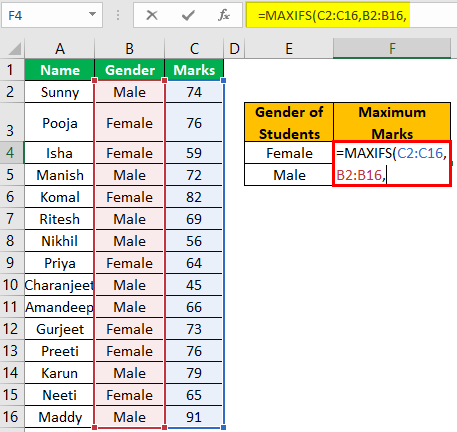
For the third argument, we will refer to the cell to the left of the formula cell. A left cell contains "Female," which is the gender which we need to compare first and then get the maximum marks.

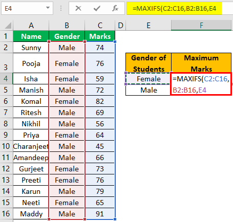
We will close the bracket for the function and get the maximum marks scored by a female student.

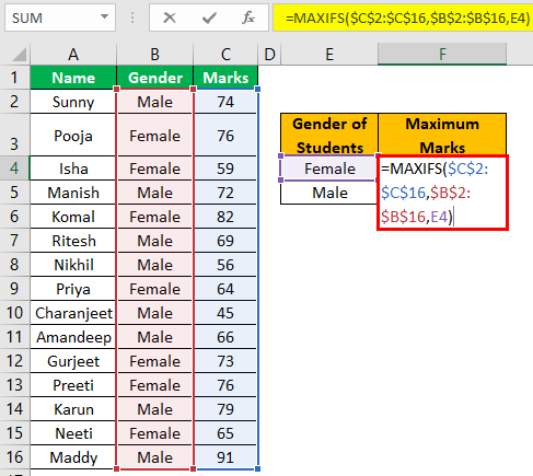
As we can see in the above function, we have used a relative cell reference in excel for all three arguments, which means that if we copy and paste the function into another cell, then the reference will get changed. So if we want to keep the reference the same, we need to use absolute reference.

We will use the ‘$’ sign before the column alphabet and row number to make reference absolute.

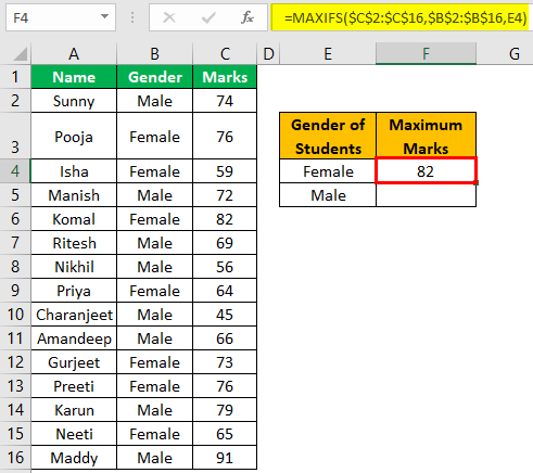
So, the maximum number of marks scored by the female student is 82.

We will copy the formula and paste it into the cell for male students. We use “Paste Formula Only” from 'Paste Special' as we do not want to copy the formatting.

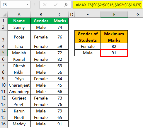
We have got the maximum marks scored by a male student, which is 91.

Example #2

In the earlier version of Excel, we do not have the MAXIFS function as a built-in function. In that case, we were using an array formula based on MAX and IF functions.

Suppose we have the following data for an organization.

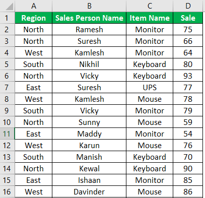
In this data, we can see that the salesperson has sold various items in different regions. Therefore, we can use an array formula based on MAX and IF functions if we want to find the maximum quantity of an item sold.

Steps:

We need to create a drop-down for item names so that the user can select from the list. In addition, he will not have to type as there can be spelling errors. To create a drop-down list in excel, we need to make the format.

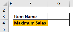
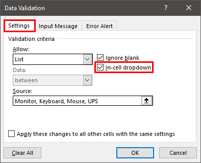
We will select the cell to create a drop-down and then click on the 'Data Validation in Excel' command available in the "Data Tools" group in the "Data."

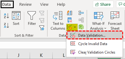
We must choose "List" for the ‘"Allow" option, type the item names in the "Source" text box, and click on "OK."

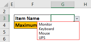
A drop-down will be created as follows:

Now to get maximum sales, we may apply the formula as follows:

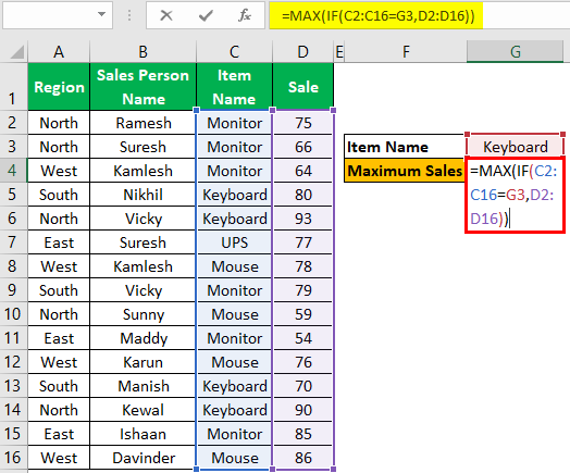
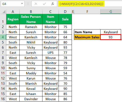
While entering the formula, we need to press Ctrl+Shift+Enter keys as this is an array formula.

As we have given a range of multiple cells for ‘logical_test’ for the IF function and have compared the same with "Item Name" written in the above cell, the IF function in excel will return more than one value, and then the MAX function will take out the maximum value. As the IF function returns more than one value, it is called an array formula in excel.

Example #3

Suppose we want to find maximum sales for an item based on the region. We will use the NESTED IF formula with the MAX function to do the same.

Steps would be:

First, we need to create the format as follows:

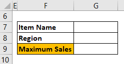
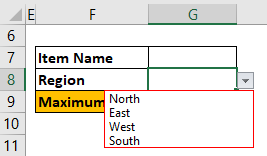
Next, we need to create a drop-down for "Item Name" and "Region."

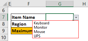
Now, we will apply the array formula based on NESTED IF in Excel and MAX function.

First, we need to compare item names with the value written in "G7" and then the region with the value written in "G8." The IF functions will return values for a particular item and region. The MAX function will return the maximum value.

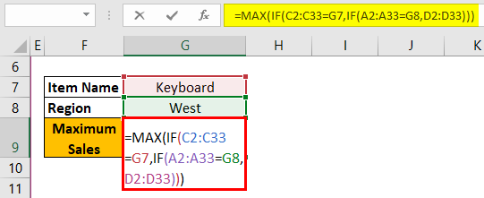
The maximum sales of "Keyboard" in the "West" region are 34.

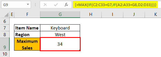
Ensure that we press Ctrl+Shift+Enter while entering the formula as this is an array formula.

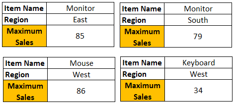
Now, we must select item names and regions to find maximum sales.

Things to Remember

We must together press the keys Control Shift-Enter in Excel while entering an array formula.
To get the maximum value, we can specify any number of conditions with nested IF functions and MAX.
The size and shape of the max_range and criteria_range N arguments must be the same. Otherwise, MAXIFS functions return the #VALUE! Error.