Search Box in Excel

Creating a Search Box in Excel

The idea of creating a search box in Excel is that we keep writing the required data. Accordingly, it will filter the data and show only that much data. This article will show you how to create a search box and filter the data in Excel.

15 Easy Steps  to Create Dynamic Search Box in Excel

To create a dynamic search box in Excel. We are going to use the below data. You can download the workbook and follow along with us to make it yourself.

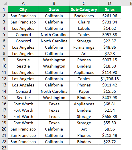
Follow the below steps to create a dynamic search box in Excel.

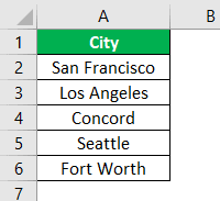
• Step 1: First, create a unique list of "City" names by removing duplicates in a new worksheet.

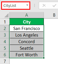
• Step 2: For this unique list of cities, give the name "CityList."

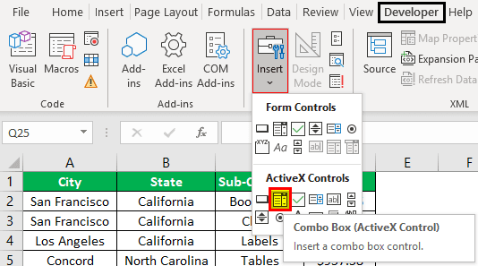
• Step 3: Go to the "Developer" tab in excel. From the "Insert" box inserts "Combo Box."

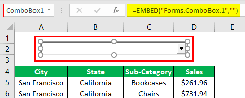
• Step 4: Draw this "ComboBox" on the worksheet where the data is.

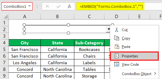
• Step 5: Right-click on this "ComboBox" and choose the "Properties" option.

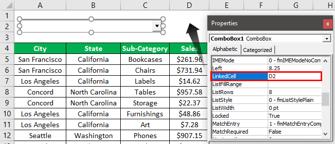
• Step 6: This will open up the "Properties" options like the below one.

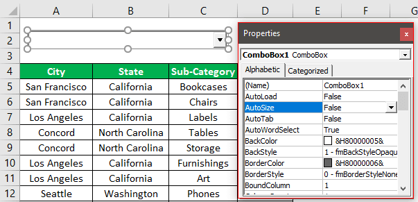
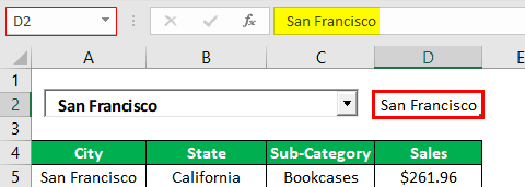
• Step 7: We have several properties here. For the property, "LinkedCell" gives a link to cell D2.

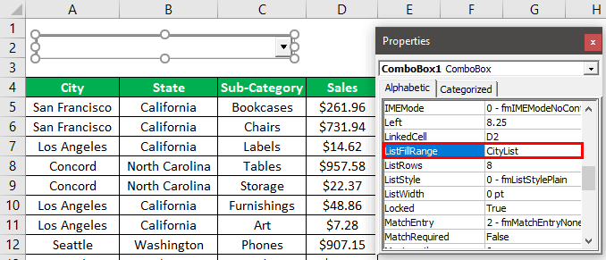
• Step 8: For the "ListFillRange," property gives the name given to a unique list of "Cities."

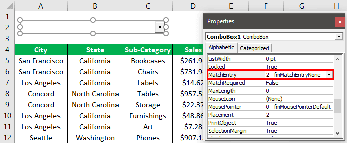
• Step 9: For the "Match Entry" property, choose "2-fmMatchEntryNone" as you type the name in the combo box. It will not auto-complete the sentence.

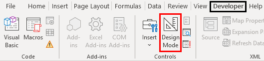
• Step 10: We are done with the properties part of "ComboBox." Go to the "Developer" tab and unselect the "Design" mode option of "Combo Box."

• Step 11: Now, from the combo box, we can see city names in the dropdown list in excel.

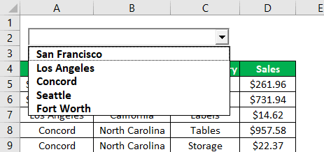
We can type the name inside the combo box, which will also reflect inlined cell D2.

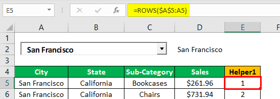
• Step 12: We need to write formulas to filter the data by typing the city name in the combo box. For this, we must have three helper columns. For the first helper column, we need to find the row numbers by using the ROWS function.

• Step 13: In the “Helper 2” column, we need to find the related search city names. If they match, we need the row numbers of those cities for this to insert the below formula.

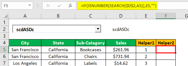
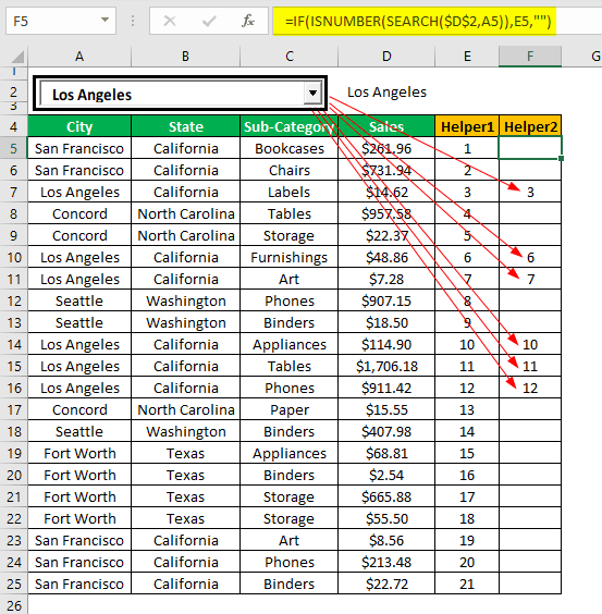
This formula will look for the city name in the main table. It will return the row number from the "Helper 1" column if it matches. Else, it will return an empty cell.

For example, now we will type "Los Angeles," and wherever the city name is in the main table for those cities, we will get the row number.

• Step 14: Once the row numbers of the entered or selected city name are available, we need to stick together these row numbers under the other. So, in the third helper column, we must stack all the entered city names row numbers.

To get these row numbers together, we will use the combination formula of the "IFERROR in Excel" and "SMALL" functions in Excel.

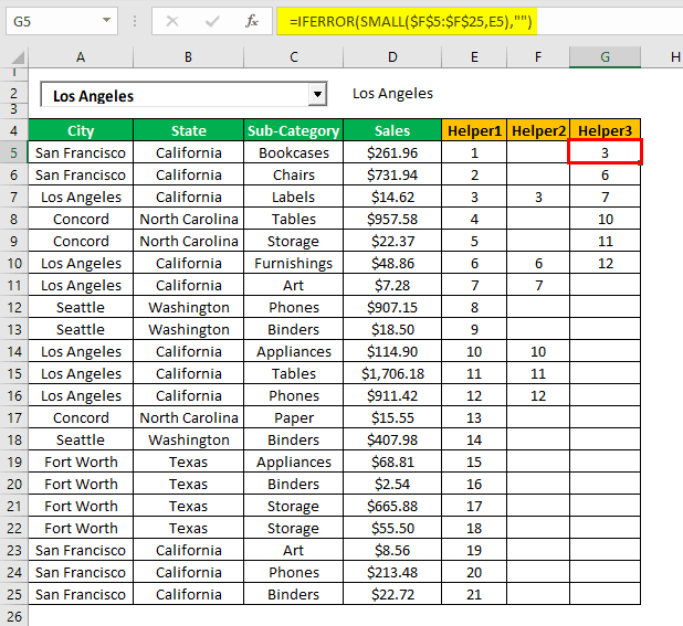
This formula will look for the smallest value in the matched city list based on actual row numbers. It will stack the first smallest, second smallest, third smallest, and so on. Once all the small values are stacked together, the SMALL function throws an error value. So, to avoid this, we have used the IFERROR function. If the error value comes, it will return an empty cell.

• Step 15: Create an identical table format like the one below.

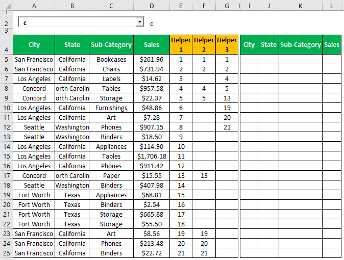
In this new table, we need to filter the data based on the city name we type in the excel search box. We can combine IFERROR, INDEX, and COLUMNS functions in excel. Below is the formula you need to apply.

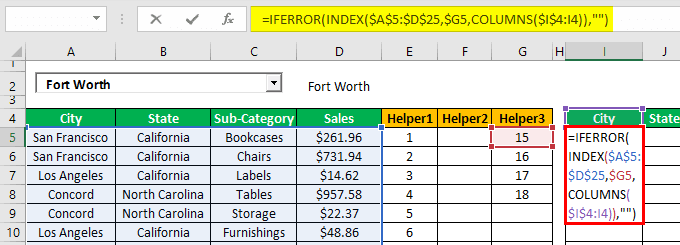
Copy the formula and paste it into all the other cells in the new table.

We are done with the designing part. Let us learn how to use it.

Please type the city name in the combo box. Our new table will only filter the entered city-data.

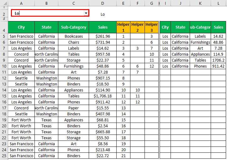
As we can see, we just typed "Lo," and all the related search results are filtered in the new table format.

Things to Remember here

• We must insert a combo box in excel from "ActiveX Form Controls" under the "Developer" tab.
• The combo box matches all the related alphabets and returns the result.

Recommended Articles

This article is a guide to the search box in Excel. Here, we discuss creating a dynamic search box in Excel along with an example and downloadable Excel templates. You may also look at these useful functions in Excel: -

• Carriage Return in Excel
• Use Form Controls in Excel
• How to Search in Excel?
• Name Box in Excel