Status Bar In Excel

Last Updated :

21 Aug, 2024

Blog Author :

Edited by :

Reviewed by :

Table Of Contents

What Is Status Bar In Excel?

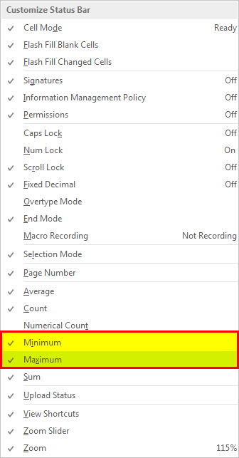
The status bar displays the status in the bottom right corner of Excel. It is a customizable bar that we can customize per the user’s needs. The status bar default has a page layout and setup view available. To customize it, we need to right-click on the status bar, and we will find various options.

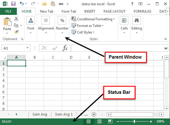
In Microsoft, every application has a status bar at the bottom of the window, which displays various options. In addition, in every application of Microsoft, there is a parent bar with all the other options of the “File,” “Insert,” etc., and a status bar on the far bottom of the window.

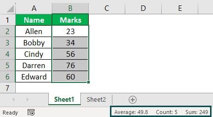
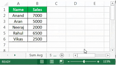
For example, consider the below table showing marks obtained by 5 students. Now, we can use the functions and formulas available in Excel to calculate average, or we can directly use the status bar.

Step 1: Select the data which has to be calculated. So, in this example, select cell range B2:B6.

As soon as we select, we can see the status bar showing the average, count, and sum values.

Likewise, we can use status bar in Excel.

What Is Status Bar In Excel?

The status bar in Excel shows the status of the selected data at the bottom right corner.
The status bar in Excel is located under the parent window.
We can customize status bar in Excel based on our needs.
It is a customizable bar that we can customize per the user’s needs.
To customize, we need to right-click on the status bar in Excel and choose from the available options.
By default, average, count, sum functions’ values can be viewed at the status bar in Excel.

How To Use Status Bar In Excel?

Let us learn the use of the status bar by a few examples.

Example #1

We will consider that the user has very little knowledge about the formulas to calculate the total marks and the average marks scored by the student in his exams.

Below are the steps of calculation of the total marks and average marks of students:

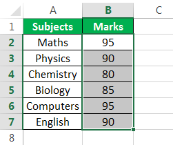
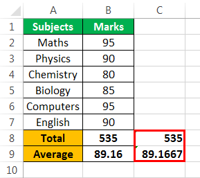
First, select the marks, which is cell B2:B7.
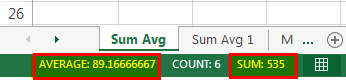
Now, have a look at the status bar. It shows us the sum and average of the marks, as we had this option checked in our status bar.
Now, while looking at this status bar, the user can input the average and total marks’ values.
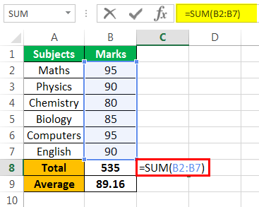
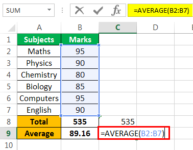
Let us calculate the average and sum by the formulas to check whether the values shown by the status bar are correct or not.
Insert the SUM function in cell C8, write down =SUM(select the range B2:B7, and press the “Enter” key.)
Also, in cell C9 write =AVERAGE( select the range B2:B7 and press the “Enter” key).
We can check that the values shown in the status bar are correct.

Example #2

Consider the following data,

It is the data for sales done by the employees of a company. Suppose the boss is having a quick look at the raw data and wants to know the sales done by each employee either in total or in a respective month or the total sales made by them in any month. Let us find out.

To know the total sales made by Anand, select cell B2:D2 and see the status bar.

Now, let us calculate the total sales done in January. So, choose cells B2:B6 and see the status bar.

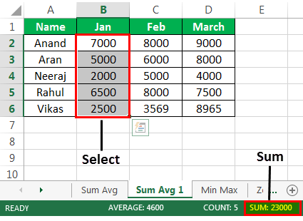
Let us find out the average sales done in all the months combined. Then, select cells B2:D6 and look at the status bar.

The status bar not only shows the sum and average or the count of selected cells. It does even show more, which we will learn in further examples.

Example #3 - Customize Status Bar

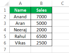
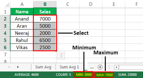
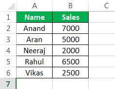
Consider the following data, which shows the total sales done by the employees of a company.

Suppose we want to know the minimum and maximum sales done.

Step 1: Enable maximum and minimum in the status bar, right-click on the status bar, and the customize dialog box appears.

Step 2: Click on “Minimum” and “Maximum.” A tick mark appears, showing that these options have been enabled.

Step 3: Now, we have the minimum and maximum options enabled. Select the data, B2:B7.

Step 4: Now, if we look at the status bar, we can see that it also shows the maximum value and minimum value selected.

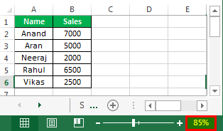
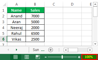
Example #4 - Zoom Option

One of the very useful tools in the status bar is the zoom option. It allows the user to zoom in or zoom out the data for a better view. Any user can adjust it according to their convenience.

Consider the following same data,

Step 1: There is a zoom slider in the bottom right of the status bar.

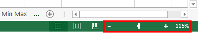
Step 2: If we click on the “plus” sign, it zooms the text in the worksheet.

Step 3: For example, take it to 150% and have a look at the data.

Step 4: Now, decrease it to 85% and look at the data.

Step 5: Any user can increase or decrease the data size. Well, the usual normal size is 100%.

Important Things To Note

We must select the appropriate options to view like, sum, average, minimum, and maximum.
To customize the data, we must right-click on the status bar.
We must select the range of data to view any status we desire.

Frequently Asked Questions (FAQs)

1. What is the status bar in Excel?

The status bar in Excel is located under the parent window, at the bottom of the application. It shows the status of the selected data.
For example, the below table shows the age of some people. Now, instead of using the functions in Excel, we can easily derive average using the status bar in Excel.

Status Bar in Excel FAQ 1

Step 1: Select the data which has to be calculated. So, in this example, select cell range B2:B6.

Status Bar in Excel FAQ 1 - Output

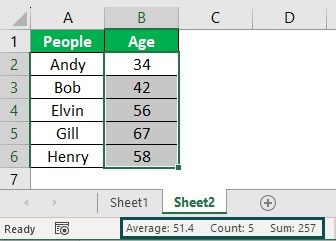
As soon as we select, we can see the status bar showing the average, count, and sum values.

Likewise, we can use status bar in Excel.

2. Where is status bar in Excel?

Like any other window application, Excel has its status bar at the bottom of the parent window.
Refer to the screenshot below,

Parent window & status Bar

With the help of the status bar, we can quickly view various things such as average, sum, minimum, maximum, etc.

3. How to customize status bar in Excel?

We can also customize the status bar. Please right-click on the status bar and click on the options we need to view quickly.

Status Bar Option

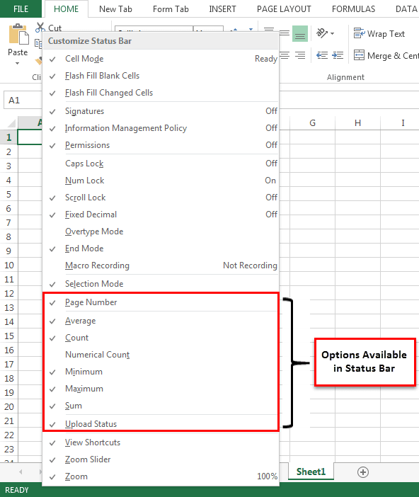
The above screenshot currently checks the average count, sum, and other options.

Download Template

This article must help understand Status Bar in Excel formulas and examples. We can download the template here to use it instantly.