Mixed References In Excel

Last Updated :

21 Aug, 2024

Blog Author :

Edited by :

Reviewed by :

Table Of Contents

What Is Mixed References In Excel?

A mixed reference in Excel is a type of cell reference different from the other two absolute and relative. We only refer to the cell's column or row in the mixed cell reference.

Mixed references are tricky referencing. A dollar sign is used before the row or the column for mixed reference. Excel Mixed reference locks the column or the row behind which the dollar sign is applied.

So, for example, in cell A1 if we want to refer to only the A column, the mixed reference would be $A1. To do this, we must press F4 on the cell twice.

What Is Mixed References In Excel?

A mixed reference in Excel is a cell reference distinct from the other two: absolute and relative. For this, one must refer to the cell’s column or row in the mixed cell reference.
One can use it for efficient data handling in relevant projects where relative or absolute referencing makes the data impossible to use.
It also acts as a helpful tool when it comes to managing data in a complex, multi-variable environment with uneven distribution, streamlining the process and making it more efficient.

Understanding Mixed Excel References

Mixed reference locks just one of the cells but not both.

In other words, part of the reference in mixed referencing is a relative, and part is absolute. We can use them to copy the formula across columns and rows, eliminating the manual need for editing. They are difficult to set up but make it easier to insert Excel formulas. They reduce errors significantly as the same formula gets copied. For example, the dollar sign, when placed before the number, then it means that it has locked the Row. Similarly, when the dollar sign is placed before the alphabet, it has locked the column.

Striking the F4 key multiple times helps change the dollar sign's position. Remember that we cannot paste mixed references into a table. We can only create an absolute or relative reference in a table. However, we can use the excel shortcut “ALT+36” or “Shift+4” key for inserting the dollar sign in Excel.

How To Use Mixed References In Excel?

Mixed references in Excel saves users time and helps in creating effective content. Let us learn how to create mixed references in Excel with the following examples.

Examples

Example #1

The easiest and simplest way of understanding mixed references is through a multiplication table in Excel.

Let us write down the multiplication table, as shown below.

The rows and columns contain the same numbers, which we will multiply.
We have inserted the multiplication formula along with the dollar sign.
The formula has been inserted, and we have copied the same formula in all the cells. We can easily copy the formula by dragging the fill handle over the cells we need to copy. Then, we can double-click on the cell to check the formula for accuracy.
We can view the formula by clicking on the "Show Formulas" command in the "Formulas" ribbon.

Looking closely at the formulas, we notice that column "B" and row "2" never change. So it is easily understood where we need to put the dollar sign.
The result of the multiplication table is shown below.

Example #2

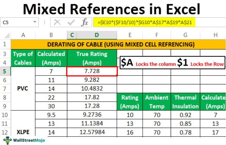
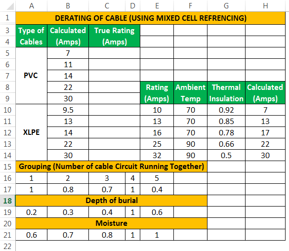
Now let us take a look at a more complicated example. The table below shows the calculation of the derating of cables in the electrical power system. The columns provide the information of the fields as follows:

Types of Cables
Calculated Current in Ampere
The details of the types of cables as:
1. Rating in Ampere
2. Ambient temperature
3. Thermal insulation
4. Calculated current in Ampere
Number of cable circuit running together
Depth of the burial of the cable
The moisture of the soil

Step 1: With the help of these data, we will calculate the true rating in ampere of the cable. These data are accumulated from the National Fire Protection Association of the USA, depending on the cable we will use. Firstly, these data are entered into the cells manually.

Step 2: We use a mixed cell reference for entering the formula in the cells from D5 to D9 and D10 to D14 independently, as shown in the snapshot.

We use the drag handle to copy the formulas in the cells.

We need to calculate the "True Rating (Amps)" from a given coefficient of "Ambient Temperature," "Thermal Insulation," and "Calculated (Amps)" currents. Here, we need to understand that we cannot calculate these by relative or absolute referencing as this will lead to miscalculations due to non-uniform data distribution. Hence, we need to use mixed referencing to resolve this because it locks the specific rows and columns according to our needs.

Step 3: We have the calculated values of a true cable rating in ampere without any miscalculation or errors.

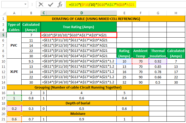
As we can see from the snapshot above, row number 17, 19, and 21 is locked by using the ‘$’ symbol. If we do not use the dollar symbol, the formula will change if we copy it to another cell as the cells are not locked, which will change the rows and columns used in the formula.

Applications Of Mixed Referencing In Excel

We can use mixed referencing for efficient data handling for our relevant projects, as explained in the above examples in which relative or absolute referencing makes the data impossible to use.
It helps us manage the data handling in a multi-variable environment where the distribution data is not uniform.

Frequently Asked Questions (FAQs)

1. What is the difference between absolute and mixed cell reference?

When formulating a spreadsheet, it is essential to reference specific cells. Cell references are of three types: absolute, relative, and mixed. Absolute references keep the cell fixed in place, while relative references change based on the cell destination. Mixed references are a combination of the two. Most formulas utilize relative and absolute references, while mixed references are less frequently used. By understanding and utilizing these referencing types, one can create practical and efficient formulas in a spreadsheet.

2. Which cell reference is a valid mixed cell reference?

In the context of valid cell referencing, coordinates that feature a dollar sign, such as $H$1 or $H$1:$H$10, are classified as absolute references. Conversely, a mixed reference involves the combination of one relative and one absolute coordinate will appear as shown in the below image.

$H1 or H$1

3. When would you use a mixed cell reference?

Mixed references are commonly used in Excel as they are helpful in situations where the same calculations are applied across rows and columns. They may be more complicated than absolute and relative references at first, but they can save time and minimize errors in the long run.