Cell Reference In Excel

A cell reference in Excel refers to other cells to a cell to use its values or properties. So in simple terms, if we have data in some random cell A2 and we want to use that value of cell A2 in cell A1, we can use =A2 in cell A1. So it will copy the value of A2 in A1. So it is called cell referencing in Excel.

For example, suppose you insert C1O. As a result, it will expand "Column C" and the "10th Row."

Likewise, we can also define or declare cell references to any location in the worksheet. We may also activate another way for cell reference.

1. Cell reference in Excel refers to a cell that is copied from another cell to use its values or properties. For example, if data is stored in a random cell A2, and the value of A2 is copied to cell A1, this is known as cell referencing.
2. Excel offers three types of cell references: relative cell references, absolute cell references, and mixed cell references.
3. Cell references are crucial in Excel functions, formulas, charts, and commands. They can be either a row or a column, but not both, and can be locked using mixed references.

• Excel worksheet is made up of cells. Each cell has a cell reference.
• Cell reference contains one or more letters or alphabet followed by a number where the letter or alphabet indicates the column and the number represents the row.
• Each cell can be located or identified by its cell reference or address, e.g., B5.
• Each cell in an Excel worksheet has a unique address. Its location on the grid defines the address of each cell. g. In the below-mentioned screenshot, the address “B5” refers to the cell in the fifth row of column B.

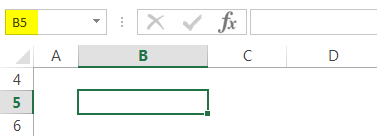
Even if we enter the cell address directly in the grid or name window, it will go to that cell location in the worksheet. Cell references can refer to either one cell, a range of cells, or even entire rows and columns.

Range Reference

Range reference in Excel is a group of cells arranged in rows or columns. In other words, when a cell reference refers to more than one cell, it is called “range.” For e.g., A1:A8 indicates the first 8 cells in column A. In between, a colon is used.

There are two types of cell reference styles in Excel. They are A1 reference and R1C1 reference.

Let us learn the difference between A1 reference and R1C1 reference.

-A1 Reference

A1 reference is the reference style, available in Excel by default. We know that, Excel is divided into rows and columns, referred with numbers and alphabets respectively. These are called row headings and column headings. A1 reference style helps users identify the cells with row and column headings.

For example, F5 refers to row 5 and column F as shown in the below image.

-R1C1 Reference

Another style of cell reference is R1C1 cell reference style. In this method, we identify cells using both row and column number. It is useful while users try to identify row and column positions in macros.

We can create a reference in Excel using simple steps. The steps are:

Step 1: Select the cell where we want to enter the formula and type equal to (=) sign.

Step 2: Now, we can directly click the cell or alternatively, we can enter the reference in the selected cell or formula box directly.

Step 3: Finally press Enter key.

For example, consider the data in cells A1 and B1. We can enter =A1+B1 in target cell C1.

Now, press Enter key. We can see the result in cell C1.

Likewise, we can create a reference.

Alternatively, we can also use the formula. For example, consider the below table showing data in cells A1 and B1.

The formula is =SUM(A1:B1).

Then, press Enter key. We can see the result in cell C1.

Likewise, we can create reference in Excel.

Now, let us learn how to change a reference in a formula.

We can change the cell address in an already available formula with the following steps.

Step 1: To begin with, we need to select the cell containing the formula. Then, double click on the cell or press the shortcut key, F2.

Step 2: Next, we can select and type the new reference in the formula. Alternatively, we can also select the reference and drag or select the additional cells or cell range.

For example, consider the below example showing the sum of two cells (A1 and B1).

Now, we can see that additionally two new data is added in cells A2 and B2. So, double click on the cell and select the cell references A2 and B2.

Now, press Enter key. We can see the result as shown in cell C1.

We have found the result. Similarly, we can use formula.

For example, consider the below example showing the sum of two cells (A1 and B1) using the formula, =SUM(A1:B1).

Now, we can see that additionally two new data is added in cells A2 and B2. Now, select the cell references A2:B2.

Now, press Enter key. We can see the result as shown in cell C1.

Likewise, we can change cell references in Excel.

Cross reference in Excel is identifying not just the target cell but also the sheet and workbook. We can use cross references from another sheet and from another workbook.

• From Another Sheet

We can select a cell or range within the same workbook and identify the sheet. The steps are:

Step 1: To start with, type the formula and click the sheet which we want to cross-reference.

Step 2: Then, press Enter key.

For example, consider the below image. Let us insert by pressing = in cell A1.

Then, click on sheet tab. In this example, let us select Example sheet tab.

We will be able to see the result as shown in the below image.

Likewise, we can use cross reference in Excel.

• From Another Workbook

Similarly, we can cross reference from another workbook. To do this, the steps are almost the same as before but we have to specify the workbook name along with the sheet tab.

#1 - Relative cell references:

It does not contain dollar signs in a row or column, e.g., A2. Relative cell reference type in Excel changes when a formula is copied or dragged to another cell. In Excel, cell referencing is relative by default. It is the most commonly used cell reference in the formula. Let us learn this method with a detailed example.

Example - Relative Cell References

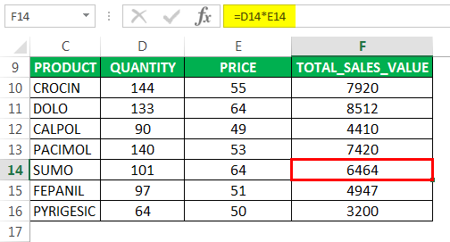
The below-mentioned pharma sales table below contains medicine "Products" in column C (C10:C16), "Quantity Sold" in column D (D10:D16), and "Total_Sales_Value" in column F, which we need to find out.

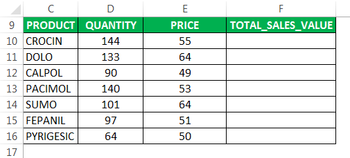
To calculate the total sales for each item, we need to multiply the price of each item by its quantity of that.

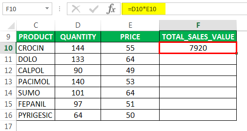
Let us check out the first item. For the first item, the formula in cell F10 would be multiplication in Excel - D10*E10.

It returns the total sales value.

Now, instead of entering the formula for all the cells, we can apply a formula to the entire range. To copy the formula down the column, click inside cell F10, and we can see that the cell is selected. Then, select the cells till F16. So, that column range will get selected. Then, we will click "Ctrl+D"to apply the formula to the entire range.

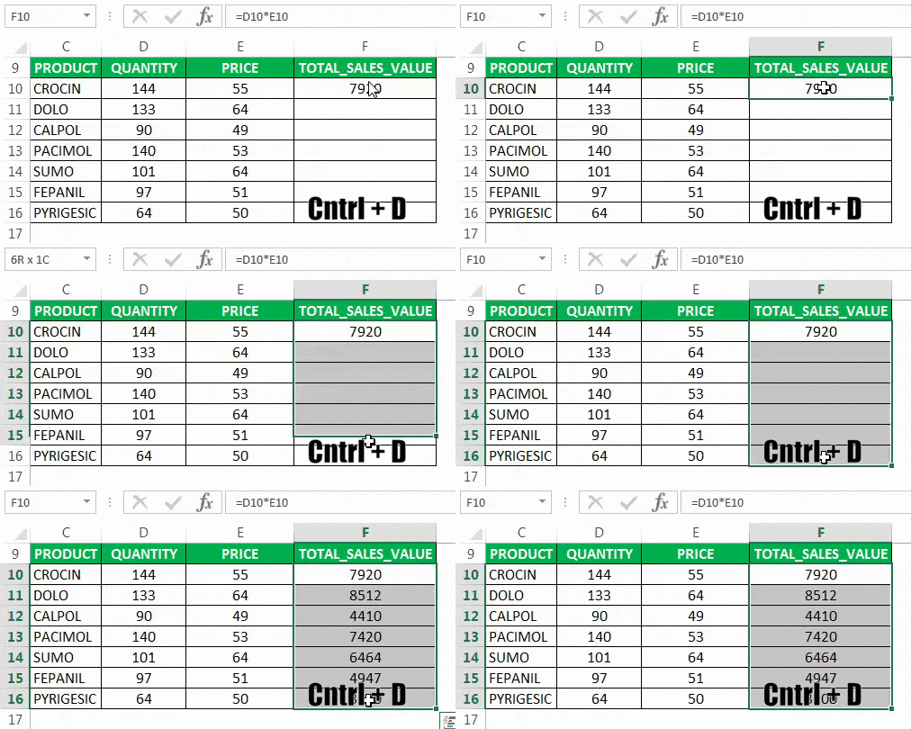
Here, when you copy or move a formula with a relative cell reference to another row. Automatically, row references will change (similarly for columns also)

We can notice that the cell reference automatically adjusts to the corresponding row.

To check a relative reference, we must select any of the cells of the "Total _Sales_ Value" in column F, and we can view the formula in the formula bar. E.g., In cell F14, we can observe that the formula has been changed from D10*E10 to D14*E14.

#2 - Absolute cell references:

Absolute cell reference contains dollar signs attached to each letter or number in a reference, e.g., $B$4. Suppose we mention a dollar sign before the column and row identifiers. It makes absolute or locks both the column and the row, i.e., where cell reference remains constant even if it is copied or dragged to another cell. Let us learn this method with a detailed example.

Example - Absolute Cell References

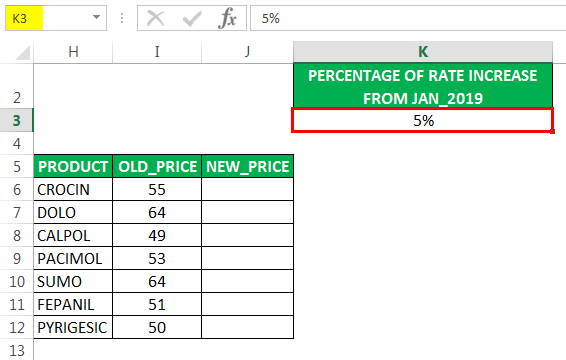
The below-mentioned pharma product table contains medicine "Products" in column H (H6:H12), and it's "Old_Price" in column I (I6:I12), and "New_Price" in column J, which we need to find out with the help of absolute cell reference.

We can see that the rate for each product is increased by 5% effective from Jan 2019 and is listed in cell "K3".

To calculate the "New_Price" for each item, we need to multiply the old price of each item by the percentage price increase (5%) and add the “Old_Price” to it.

Let us check out the first item. For the first item, the formula in cell J6 would be =I6*$K$3+I6, where it returns the new price.

Here, the percentage rate increase for each product is 5%, a common factor. Therefore, we must add a dollar symbol in front of the row and column number for the cell "K3" to make it an absolute reference, i.e., $K$3.Wecan add it by clicking the "function+F4" key once.

Here the dollar sign for the cell "K3" fixes the reference to a given cell, where it remains unchanged no matter when you copy or apply a formula to other cells.

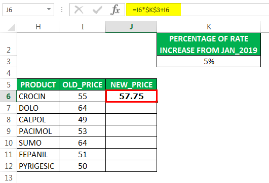
Here, $K$3 is an absolute cell reference, whereas "I6" is a relative cell reference. It changes when you apply to the next cell.

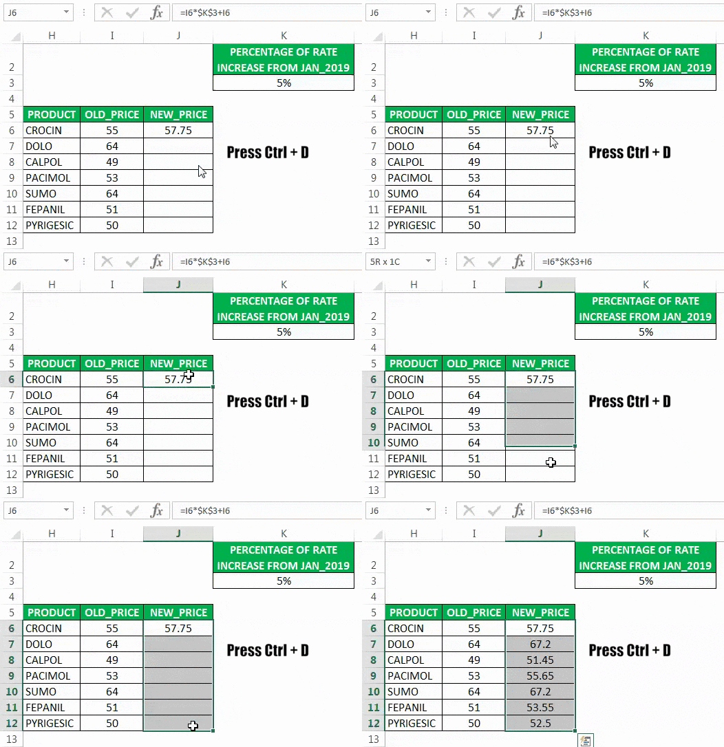
Now, instead of entering the formula for all the cells, we can apply a formula to the entire range. To copy the formula down the column, click inside cell J6, and we will see that the cell has been selected. Then, we must select the cells till J12. So, that column range will get selected. Then click "Ctrl+D," so the formula is applied to the entire range.

#3 - Mixed cell references in Excel:

In Excel, mixed cell references contain dollar signs attached to either the letter or the number in a reference. E.g., $B2 or B$4. It is a combination of relative and absolute references. Let us learn this method with a detailed example.

Example - Mixed Cell References

In the below-mentioned table, we have values in each row (D22, D23, and D24) and columns (E21, F21, and G21). Here, we have to multiply each column with each row with the help of a mixed cell reference.

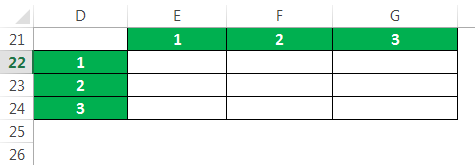
There are two types of mixed cell references that we can use here to get the desired output.

Let us apply two types of mixed references below in the cell "E22."

The formula would be =$D22*E$21.

#1 - $D22: Absolute column and Relative row

Here, the dollar sign before column D indicatesthat only the row number can change. At the same time, the column letter D is fixed. It does not change.

When we copy the formula to the right side, the reference will not change because it is locked, but When you copy it down, the row number will change because it is not locked.

#2 - E$21: Absolute row and Relative column

Consider the below example.

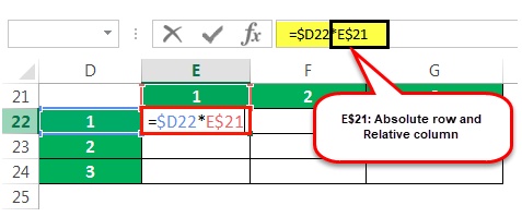
The dollar sign right before the row number indicates only the column letter E can change. Whereas the row number is fixed; it does not change.

The row number will not change when copying the formula because it is locked. But when we copy the formula to the right side, the column alphabet will change because it is not locked.

Now, instead of entering the formula for all the cells, we can apply a formula to the entire range. Now, we will click inside cell E22. As a result, first, we will see that the cell is selected. Then, we will select the cells until G24 so that the entire range will get selected. Next, we will click on the "Ctrl+D" key first and later "Ctrl+R."

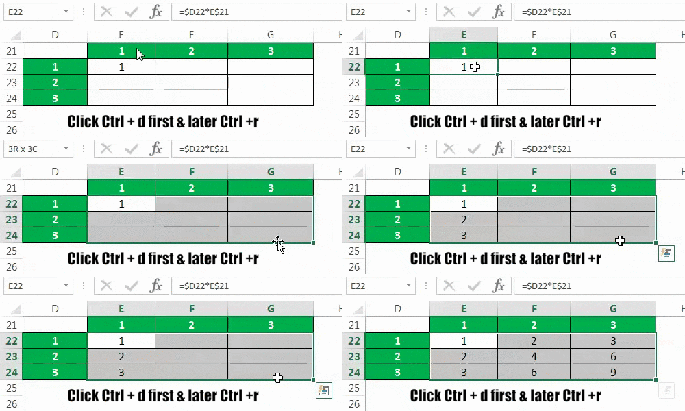
Likewise, we can use cell references in Excel.

Throughout this article, we saw how to create and change the cell reference in Excel. In this section, let us learn how to switch or change the cell reference type.

The steps are:

Step 1: To begin with, select the cell with the formula. In the formula bar, we need to select the reference we want to change.

Step 2: Now, we have to press the shortcut key, F4 to change the reference type.

Circular Reference

The circular reference in Excel, as the name suggests is a type of cell reference where the same cell is referred back. It is advised not to use this reference type as we may get errors in our sheet.

• The cell reference is a key element of formula or excels functions.
• Cell references are used in Excel functions, formulas, charts, and other Excel commands.
• Mixed reference locks either one. It may be a row or column, but not both.