What Is Circular Reference In Excel?
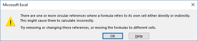
A Circular Reference in Excel occurs is when a formula in a cell refers to its cell. A Circular Reference is an error message revealed by Excel, to denote that we are using a Circular Reference in our formula and the output calculated is incorrect.
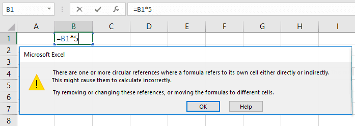
For example, in cell B1, if we write a formula =B1*5, this is a Circular Reference as inside cell B1, we used the cell reference to B1 itself.
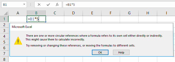
As we see in the image above, cell B1 straightforwardly refers to its very own cell, which is not possible. So, we get the error, i.e., creates a Circular Reference, and shows a warning that found one or more Circular References.
Key Takeaways
- The Circular Reference in Excel occurs when an equation in a cell that specifically or in a roundabout way refers to its very own cell.
- We can type the smallest number under the Maximum Change Value to proceed with the Circular Reference. The smaller the number, the more precise the result, and the more time Excel will take to calculate a worksheet.
- When we open the file again after saving, it also shows the warning message that one or more formula contains a Circular Reference. Therefore, ensure to check that Circular Reference is enabled.
How To Use Circular Reference In Excel?
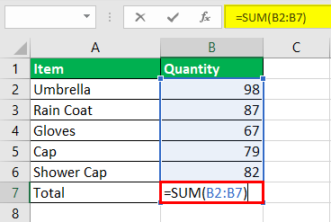
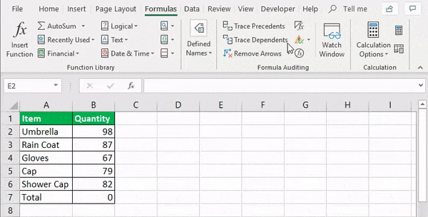
In the data given below, we have already got the result as 0, for the formula =SUM(B2:B7) in cell B7, as the result cell is also included in the formula.
The steps to get the accurate result are,
- Step 1: We must first get the total quantity of the sold items, including the cell in which we are using the formula.
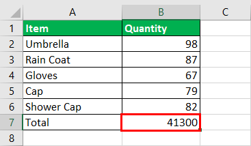
- Step 2: The cell which contains the total value returned to 41,300 instead of 413 as we enabled iterative calculation, as shown below.
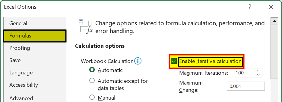
How To Enable/Disable Circular References In Excel?
If we want circular formulas to work, we mustEnableCircular Referencesin your Excel worksheet.
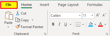
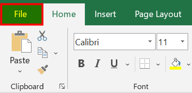
- Firstly, we must go to the “File” tab.

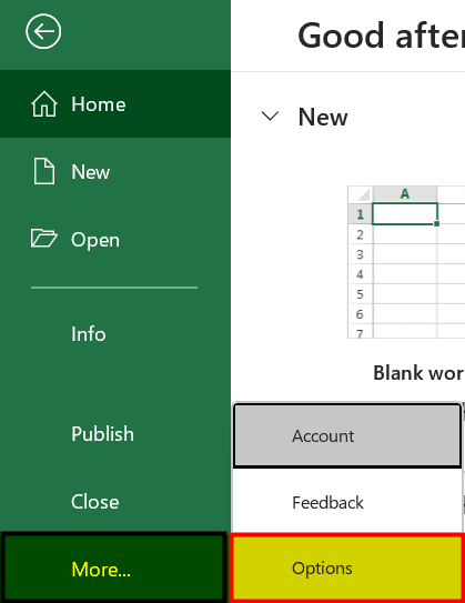
- Then, click on “Options.”

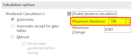
- Next, select the “Formulas” on the left, then on the right, under the “Calculation options” category, check/tick the “Iterative Calculation” checkbox, and click “OK.”

- Once you turn on the “Iterative Calculation” option in the “Formulas” tab, check and specify the options as mentioned below:
•Maximum Iterations:It indicates how often the equation ought to recalculate. The higher the number of emphases, the additional time the computation takes.•Maximum Change:It determines the most extreme change between figuring results. The smaller the number, the more precise the outcome we get and the additional time Excel takes to ascertain the worksheet.We can change the maximum iteration and maximum change as per our requirements.


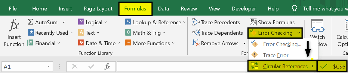
How To Find Circular References In Excel?
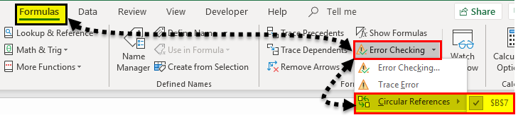
- In the above data, to find a Circular Reference, we must first go to the “Formulas” tab, then click the option bolt by “Error Checking,” and then go to “Circular References,” the last entered Circular Reference is shown here:
- Next, we must tap on the cell in the “Circular References.” Again, Excel will convey you precisely to that cell.
- When we do this, the status bar will tell us that Circular References are found in our exercise manual and show the location of one of those cells:

- If we find a Circular Reference in another Excel sheet, it only shows a cell reference.
- When we open the file again after saving, it also shows the warning message that one or more formula contains a Circular Reference.
Why Circular References Should Be Avoided?
The Excel Circular References is not recommended because it is not a methodology that we can use quickly and helps to reduce our efforts. Aside from execution issues and a notice message shown on each exercise manual opening (except if iterative estimations are on), Circular References can prompt various problems that are not quickly evident.
# Outcomes
- The arrangement joins, which implies a steady final product is to come. It is an alluring condition.
- The arrangement wanders, implying that the contrast between the current and the past outcome increments from emphasis to cycle.
- The arrangement switches between two values. For instance, once the iteration starts, the result is 1 the first time, then 10, 100, and so on, depending on the “Maximum Iterations” selected.
Remove Circular References
In the above data, to find a Circular Reference, we must first go to the “Formulas” tab, then click the option bolt by “Error Checking,” and then go to “Circular References,” the last entered Circular Reference is shown here:

Once we locate the cell, to Remove Circular References, we must alter the cell. Therefore, either delete the formula and the result, or change it with any other value which removes the formulas automatically. It will now remove the circular reference. Now, repeat this for each cell with the Circular References cells we want to remove. Removing circular references from formulas will allow Excel to correctly return a result.
Important Things To Note
- Excel does not show the notification message repeatedly when we use more than one formula in Excel with a Circular Reference.
- While using Circular Reference, we must always check that iterative calculation in the Excel sheet is enabled. Otherwise, we would not be able to use Circular References.
- Using the Circular Reference may slow down our computer because it causes our function to be repetitive until a particular condition is met.
Frequently Asked Questions (FAQs)
How to find hidden Circular Reference in Excel?
The Circular references won’t be found or are hidden, when Excel tries to recalculate formulas result that’s already been once calculated.
In such scenarios, we do not get a warning message from Excel of conditional circular references. We can still find the hidden Circular Reference in Excel.
First, select the “Formulas” tab → go to the “Formula Auditing” group → click the “Error Checking” option drop-down → select the “Circular References” option right-arrow, as shown below.
When we select that option, all the available Circular Reference cell names will appear on the right, as seen in the example above.
How do I turn off the Circular Reference warning in Excel?
When we get the error message for Circular Reference, to come out of the warning message, we can click “Help” for more data, or close the message window by clicking either “OK”, or the cross mark on the dialog box. When we close the message window, Excel may show a zero (0) or the last determined incentive in the selected cell.
How do I turn off the Circular Reference warning in Excel?
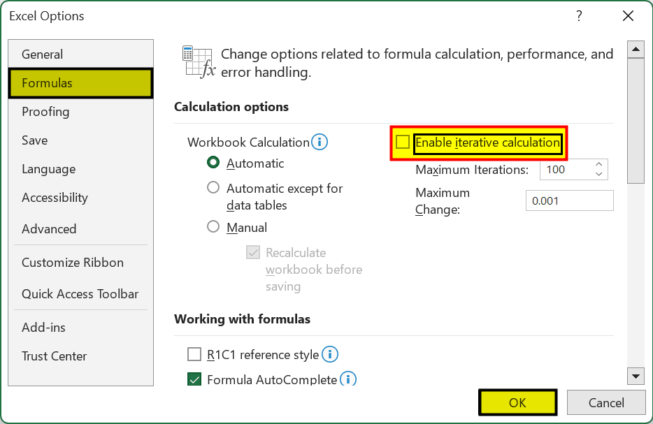
The steps to disable the Circular Reference in Excel are as follows:
1) Firstly, we must go to the “File” tab.
2) Then, click on “Options.”
3) The “Excel Options” window appears. Go to the “Formulas” on the left, then on the right, under the “Calculation options” category, we see that the “Iterative Calculation” option is checked, as shown below.
4) Uncheck the “Iterative Calculation” option, and click “OK” to remove the Circular Reference, as shown below.
Recommended Articles
This article is a guide to Circular Reference in Excel. Here we find references, enable iterative calculation as a workaround, examples, downloadable template. You can also look at our other suggested articles: –