Top 15 Financial Functions in Excel

Top 15 Financial Functions in Excel

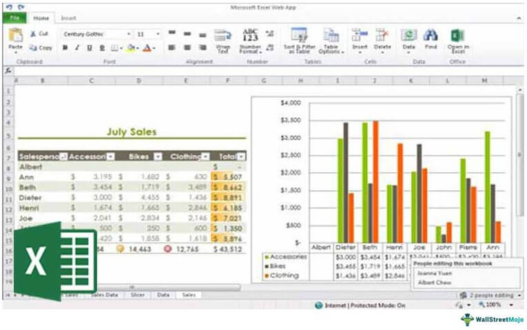
Microsoft Excel is the most important tool of  Investment Bankers and Financial Analysts. They spent more than 70% of the time preparing Excel Models, formulating Assumptions, Valuations, Calculations, Graphs, etc. It is safe to assume that Investment bankers are masters in excel shortcuts and formulas. Though there are more than 50+ Financial Functions in Excel, here is the list of Top 15 financial functions in excel that are most frequently used in practical situations.

Without much ado, let’s have a look at all the financial functions one by one –

• #1 – Future Value (FV)
• #2 – FVSCHEDULE
• #3 – Present Value (PV)
• #4 – Net Present Value (NPV)
• #5 – XNPV
• #6 – PMT
• #7 – PPMT
• #8 – Internal Rate of Return (IRR)
• #9 – Modified Internal Rate of Return (MIRR)
• #10 – XIRR
• #11 – NPER
• #12 – RATE
• #13 – EFFECT
• #14 – NOMINAL
• #15 – SLN

#1 – Future Value (FV): Financial Function in Excel 

If you want to find out the future value of a particular investment which has a constant interest rate and periodic payment, use the following formula –

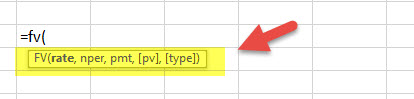
FV (Rate, Nper, [Pmt], PV, [Type])

• Rate = It is the interest rate/period
• Nper = Number of periods
• [Pmt] = Payment/period
• PV = Present Value
• [Type] = When the payment is made (if nothing is mentioned, it’s assumed that the payment has been made at the end of the period)

FV Example

A has invested the US $100 in 2016. The payment has been made yearly. The interest rate is 10% p.a. What would be the FV in 2019?

Solution: In excel, we will put the equation as follows –

= FV (10%, 3, 1, – 100)

= US $129.79

#2 – FVSCHEDULE: Financial Function in Excel 

This financial function is important when you need to calculate the future value with the variable interest rate. Have a look at the function below –

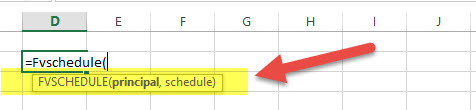
FVSCHEDULE = (Principal, Schedule)

• Principal = Principal is the present value of a particular investment
• Schedule = A series of interest rate put together (in case of excel, we will use different boxes and select the range)

FVSCHEDULE Example:

M has invested the US $100 at the end of 2016. It is expected that the interest rate will change every year. In 2017, 2018 & 2019, the interest rates would be 4%, 6% & 5% respectively. What would be the FV in 2019?

Solution: In excel, we will do the following –

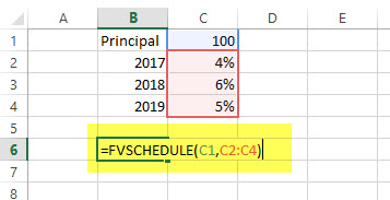
= FVSCHEDULE (C1, C2: C4)

= US $115.752

#3 – Present Value (PV): Financial Function in Excel 

If you know how to calculate FV, it’s easier for you to find out PV. Here’s how –

PV = (Rate, Nper, [Pmt], FV, [Type])

• Rate = It is the interest rate/period
• Nper = Number of periods
• [Pmt] = Payment/period
• FV = Future Value
• [Type] = When the payment is made (if nothing is mentioned, it’s assumed that the payment has been made at the end of the period)

PV Example:

The future value of an investment in the US $100 in 2019. The payment has been made yearly. The interest rate is 10% p.a. What would be the PV as of now?

Solution: In excel, we will put the equation as follows –

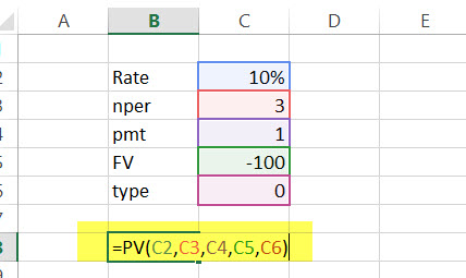
= PV (10%, 3, 1, – 100)

= US $72.64

#4 – Net Present Value (NPV): Financial Function in Excel 

Net Present Value is the sum total of positive and negative cash flows over the years. Here’s how we will represent it in excel –

NPV = (Rate, Value 1, [Value 2], [Value 3]…)

• Rate = Discount rate for a period
• Value 1, [Value 2], [Value 3]… = Positive or negative cash flows
• Here, negative values would be considered as payments, and positive values would be treated as inflows.

NPV Example

Here is a series of data from which we need to find NPV –

Details	In US $
Rate of Discount	5%
Initial Investment	-1000
Return from 1st year	300
Return from 2nd year	400
Return from 3rd year	400
Return from 4th year	300

Find out the NPV.

Solution: In Excel, we will do the following –

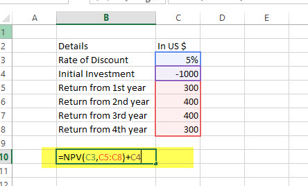
=NPV (5%, B4:B7) + B3

= US $240.87

Also, have a look at this article – NPV vs IRR

#5 – XNPV: Financial Function in Excel 

This financial function is similar to the NPV with a twist. Here the payment and income are not periodic. Rather specific dates are mentioned for each payment and income. Here’s how we will calculate it –

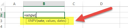
XNPV = (Rate, Values, Dates)

• Rate = Discount rate for a period
• Values = Positive or negative cash flows (an array of values)
• Dates = Specific dates (an array of dates)

XNPV Example

Here is a series of data from which we need to find NPV –

Details	In US $	Dates
Rate of Discount	5%
Initial Investment	-1000	1st December 2011
Return from 1st year	300	1st January 2012
Return from 2nd year	400	1st February 2013
Return from 3rd year	400	1st March 2014
Return from 4th year	300	1st April 2015

Solution: In excel, we will do as follows –

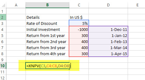
=XNPV (5%, B2:B6, C2:C6)

= US$289.90

#6 – PMT: Financial Function in Excel 

In excel, PMT denotes the periodical payment required to pay off for a particular period of time with a constant interest rate. Let’s have a look at how to calculate it in excel –

PMT = (Rate, Nper, PV, [FV], [Type])

• Rate = It is the interest rate/period
• Nper = Number of periods
• PV = Present Value
• [FV] = An optional argument which is about the future value of a loan (if nothing is mentioned, FV is considered as “0”)
• [Type] = When the payment is made (if nothing is mentioned, it’s assumed that the payment has been made at the end of the period)

PMT Example

The US $1000 needs to be paid in full in 3 years. The interest rate is 10% p.a. and the payment needs to be done yearly. Find out the PMT.

Solution: In excel, we will calculate it in the following manner –

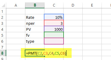
= PMT (10%, 3, 1000)

= – 402.11

#7 – PPMT: Financial Function in Excel 

It is another version of PMT. The only difference is this – PPMT calculates payment on principal with a constant interest rate and constant periodic payments. Here’s how to calculate PPMT –

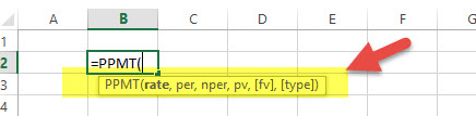
PPMT = (Rate, Per, Nper, PV, [FV], [Type])

• Rate = It is the interest rate/period
• Per = The period for which the principal is to be calculated
• Nper = Number of periods
• PV = Present Value
• [FV] = An optional argument which is about the future value of a loan (if nothing is mentioned, FV is considered as “0”)
• [Type] = When the payment is made (if nothing is mentioned, it’s assumed that the payment has been made at the end of the period)

PPMT Example

The US $1000 needs to be paid in full in 3 years. The interest rate is 10% p.a. and the payment needs to be done yearly. Find out the PPMT in the first year and second year.

Solution: In excel, we will calculate it in the following manner –

1^st year,

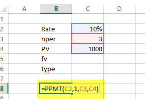
=PPMT (10%, 1, 3, 1000)

= US $-302.11 

2^nd year,

=PPMT (10%, 2, 3, 1000)

= US $-332.33

#8 – Internal Rate of Return (IRR): Financial Function in Excel 

To understand whether any new project or investment is profitable or not, the firm uses IRR. If IRR is more than the hurdle rate (acceptable rate/ average cost of capital), then it’s profitable for the firm and vice-versa. Let’s have a look, how we find out IRR in excel –

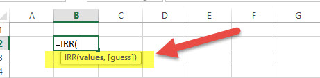
IRR = (Values, [Guess])

• Values = Positive or negative cash flows (an array of values)
• [Guess] = An assumption of what you think IRR should be

IRR Example

Here is a series of data from which we need to find IRR –

Details	In US $
Initial Investment	-1000
Return from 1st year	300
Return from 2nd year	400
Return from 3rd year	400
Return from 4th year	300

Find out IRR.

Solution: Here’s how we will calculate IRR in excel –

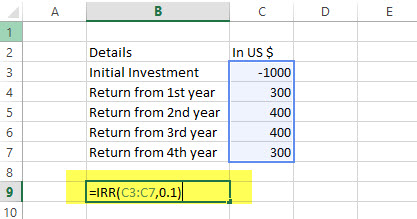
= IRR (A2:A6, 0.1)

= 15%

#9 – Modified Internal Rate of Return (MIRR): Financial Function in Excel 

The Modified Internal Rate of Return is one step ahead of the Internal Rate of Return. MIRR signifies that the investment is profitable and is used in business. MIRR is calculated by assuming NPV as zero. Here’s how to calculate MIRR in excel –

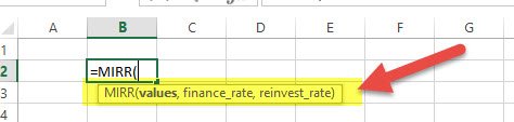
MIRR = (Values, Finance rate, Reinvestment rate)

• Values = Positive or negative cash flows (an array of values)
• Finance rate = Interest rate paid for the money used in cash flows
• Reinvestment rate = Interest rate paid for reinvestment of cash flows

MIRR Example

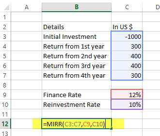
Here is a series of data from which we need to find MIRR –

Details	In US $
Initial Investment	-1000
Return from 1st year	300
Return from 2nd year	400
Return from 3rd year	400
Return from 4th year	300

Finance rate = 12%; Reinvestment rate = 10%. Find out IRR.

Solution: Let’s look at the calculation of MIRR –

= MIRR (B2:B6, 12%, 10%)

= 13%

#10 – XIRR: Financial Function in Excel 

Here we need to find out IRR, which has specific dates of cash flow. That’s the only difference between IRR and XIRR. Have a look at how to calculate XIRR in excel financial function –

XIRR = (Values, Dates, [Guess])

• Values = Positive or negative cash flows (an array of values)
• Dates = Specific dates (an array of dates)
• [Guess] = An assumption of what you think IRR should be

XIRR Example

Here is a series of data from which we need to find XIRR –

Details	In US $	Dates
Initial Investment	-1000	1st December 2011
Return from 1st year	300	1st January 2012
Return from 2nd year	400	1st February 2013
Return from 3rd year	400	1st March 2014
Return from 4th year	300	1st April 2015

Solution: Let’s have a look at the solution –

= XIRR (B2:B6, C2:C6, 0.1)

= 24%

#11 – NPER: Financial Function in Excel 

It is simply the number of periods one requires to pay off the loan. Let’s see how we can calculate NPER in excel –

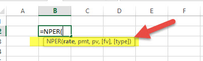
NPER = (Rate, PMT, PV, [FV], [Type])

• Rate = It is the interest rate/period
• PMT = Amount paid per period
• PV = Present Value
• [FV] = An optional argument which is about the future value of a loan (if nothing is mentioned, FV is considered as “0”)
• [Type] = When the payment is made (if nothing is mentioned, it’s assumed that the payment has been made at the end of the period)

NPER Example

US $200 is paid per year for a loan of US $1000. The interest rate is 10% p.a. and the payment needs to be done yearly. Find out the NPER.

Solution: We need to calculate NPER in the following manner –

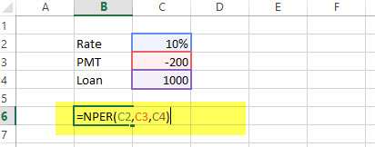
= NPER (10%, -200, 1000)

= 7.27 years

#12 – RATE: Financial Function in Excel 

Through the RATE function in excel, we can calculate the interest rate needed to pay off the loan in full for a given period of time. Let’s have a look at how to calculate RATE financial function in excel –

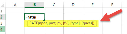
RATE = (NPER, PMT, PV, [FV], [Type], [Guess])

• Nper = Number of periods
• PMT = Amount paid per period
• PV = Present Value
• [FV] = An optional argument which is about the future value of a loan (if nothing is mentioned, FV is considered as “0”)
• [Type] = When the payment is made (if nothing is mentioned, it’s assumed that the payment has been made at the end of the period)
• [Guess] = An assumption of what you think RATE should be

RATE Example

US $200 is paid per year for a loan of US $1000 for 6 years, and the payment needs to be done yearly. Find out the RATE.

Solution:

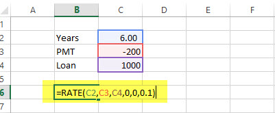
= RATE (6, -200, 1000, 0.1)

= 5%

#13 – EFFECT: Financial Function in Excel 

Through the EFFECT function, we can understand the effective annual interest rate. When we have the nominal interest rate and the number of compounding per year, it becomes easy to find out the effective rate. Let’s have a look at how to calculate EFFECT financial function in excel –

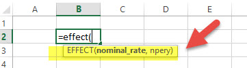
EFFECT = (Nominal_Rate, NPERY)

• Nominal_Rate = Nominal Interest Rate
• NPERY = Number of compounding per year

EFFECT Example

Payment needs to be paid with a nominal interest rate of 12% when the number of compounding per year is 12.

Solution:

= EFFECT (12%, 12)

= 12.68%

#14 – NOMINAL: Financial Function in Excel 

When we have an effective annual rate and the number of compounding periods per year, we can calculate the NOMINAL rate for the year. Let’s have a look at how to do it in excel –

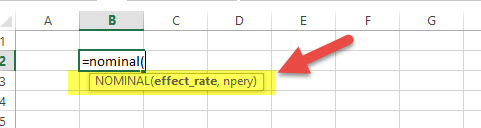
NOMINAL = (Effect_Rate, NPERY)

• Effect_Rate = Effective annual interest rate
• NPERY = Number of compounding per year

NOMINAL Example

Payment needs to be paid with an effective interest rate or annual equivalent rate of 12% when the number of compounding per year is 12.

Solution:

= NOMINAL (12%, 12)

= 11.39%

#15 – SLN: Financial Function in Excel 

Through the SLN function, we can calculate depreciation via a straight-line method. In excel, we will look at SLN financial function as follows –

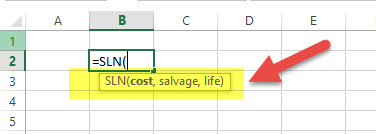
SLN = (Cost, Salvage, Life)

• Cost = Cost of an asset when bought (initial amount)
• Salvage = Value of asset after depreciation
• Life = Number of periods over which the asset is being depreciated

SLN Example

The initial cost of machinery is US $5000. It has been depreciated in the Straight Line Method. The machinery was used for 10 years, and now the salvage value of the machinery is the US $300. Find depreciation charged per year.

Solution:

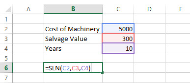
= SLN (5000, 300, 10)

= US $470 per year

You may also look at Depreciation Complete Guide

Top 15 Financial Functions in Excel Video

Recommended Articles

• PMT Formula in Excel
• Covariance Matrix in Excel
• NPER Function in Excel
• Running Total in Excel