What are Excel Shortcuts?
An Excel shortcut is a technique of performing a manual task in a quicker way. The shortcuts help speed up the work, which saves time for the secondary tasks of the job. Since Excel is used by almost everybody in some form or the other, it is essential to be aware of the shortcuts.
For example, the excel shortcut “Ctrl+O” opens an already existing workbook. The shortcut “Ctrl+W” closes the currently active workbook.
The purpose of using an excel shortcut is to save the worksheet creator from extra clicks. This improves the productivity at the workplace.
At times, the same task is repeated in Excel on a daily basis. Since such tasks may not have a shortcut, the solution is to create it by recording a macro.
Top 20 Keyboard Shortcuts in Excel
This article discusses the important excel shortcuts which have been consolidated keeping in mind the day-to-day needs of the user. The explanation of each technique is followed by a relevant example.
It is not possible to memorize every excel shortcut. However, a regular usage does allow gradual learning. To develop expertise in Excel, it is imperative to go beyond the basic cut (Ctrl+X), copy (Ctrl+C), and paste (Ctrl+V) shortcuts.
#1–Paste as Values With “Paste Special”
If a formula cell is copied and pasted, its formula is pasted and not the value of the cell. With “paste special,” it is possible to paste the value of the formula cell at the desired location.
The excel shortcut “Alt+E+S+V” (press one by one) opens the “paste special” window and selects “values” under “paste.”
Note: Prior to pressing the excel shortcut, the formula cell must be copied and the desired output cell (where output is required) should be selected.

Example
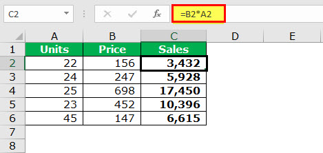
The succeeding table shows the prices (in $ in column B) at which some units (column A) of a product are sold. We want to calculate the sales figures and, instead of formulas, paste the final values in column C.
Use the shortcut of the “paste special” property.
The steps to calculate sales and apply the “paste special” shortcut are listed as follows:
Step 1: In cell C2, enter the following formula.
“=B2*A2”
The cell C2 is dependent on the cells A2 and B2.
Copy-paste or drag the formula to the remaining cells. The formulas are applied to the entire range (C2:C6).
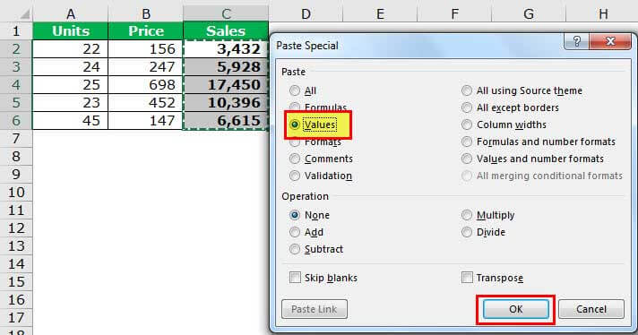
Step 2: Copy the formula cell C2. Press the keys “ALT+E+S+V” one by one. The “paste special” window opens. “Values” is automatically selected under “paste.” Click “Ok.”
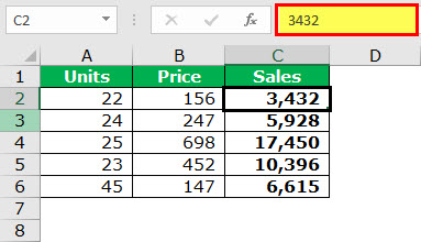
Step 3: The number 3,432 is pasted in cell C2 as a value and not as a formula.
#2–Sum Numbers With AutoSum
Often, there is a need to sum a set of numbers. To do this, we usually apply the SUM function. An alternative method is to use the excel shortcut key.
The shortcut “Alt+=” (press together) sums numbers.

Example #2
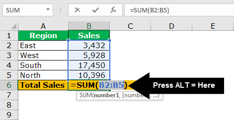
The following table shows the region-wise sales of an organization. We want to sum all the sales figures to find the total sales. Use the shortcut of AutoSum.
Step 1: Select cell B6. Press the excel shortcut keys “Alt+=” together.
Step 2: The SUM formula automatically appears in cell B6, as shown in the following image.
#3–Fill the Subsequent Cell With the Fill Down
The fill down property fills the present (subsequent) cell with the value or formula of the immediately preceding cell. This feature is often used while entering data in Excel.
The excel shortcut “Ctrl+D” (press together) fills the immediately following cell with the data or formula of the preceding cell.
If a range of cells is selected, the content of the topmost cell is filled in the cells below. If the subsequent cell already contains a value, pressing “Ctrl+D” overwrites it.
Note 1: If the preceding cell contains a value, the fill down feature copies the same to the immediately following cell. However, if the preceding cell contains a formula, the same is copied.
Note 2: While copying a formula, the cell references may or may not change depending on the kind of references used (relative or absolute).
Note 3: The shortcut “Ctrl+D” works only for columns and not for rows. For rows, use the shortcut “Ctrl+R” (press together), which fills cells to the right.

Example
The left side of the following image shows the first and the last names in columns A and B respectively. We want to copy the first name of row 4 in row 5 with the help of the fill down excel shortcut.
Step 1: Select cell A5. Press the keys “Ctrl+D” together.
Step 2: The name “Jawahar” is copied to cell A5, as shown by the right side of the following image.

Example
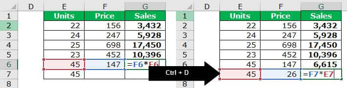
The left side of the following image shows the sales (column G) calculated by multiplying the price (column F) with the number of units (column E).
We want to calculate the sales (units=45 and price=26) for the entry in row 7. Use the fill down shortcut.
Step 1: Enter 26 as the price in cell F7. Select cell G7 and press the keys “Ctrl+D.”
Step 2: The formula of the preceding cell (G6) is copied to cell G7, as shown by the right side of the following image.
#4–Select the Entire Row or Column
Often, there is a need to select the entire row or column in Excel.
The excel shortcut “Shift+space” (press together) selects the entire row.

The shortcut “Ctrl+space” (press together) selects the entire column.

Example
The following image shows a blank worksheet. With the help of the shortcut, we want to:
a) Select row 4 in the given worksheet
b) Select column B in the given worksheet
a) Step 1: Select any cell in row 4. Press the excel shortcut keys “Shift+space” together.
Step 2: The entire row 4 is selected, as shown in the following image.
b) Step 1: Select any cell in column B. Press the shortcut keys “Ctrl+space” together.
Step 2: The entire column B is selected, as shown in the following image.
#5–Insert and Delete Row or Column
At times, we may need to insert or delete a row or column.
The excel shortcut “Ctrl+Shift+plus sign (+)” inserts a new row or column. The keys must be pressed together.
Prior to pressing this shortcut, select the entire row or column preceding which the insertion has to be made. For this, click the row or column label appearing at the leftmost side or on top.

The excel shortcut “Ctrl+minus sign (-)” deletes an existing row or column. The keys must be pressed together.
Prior to pressing this shortcut, select the entire row or column which has to be deleted.

Note: If the preceding shortcuts (insert or delete) are pressed by selecting a cell rather than the entire row or column, the “insert” or “delete” dialog box opens.
Example
The following image shows the number of units (column E), prices (column F), and sales (column G). With the help of the shortcut, we want to:
a) Insert a row preceding row 4
b) Delete the newly inserted row 4.
a) Step 1: Select the entire row 4 by clicking the label “4” at the leftmost side.
Step 2: Press the keys “Ctrl+Shift+plus sign (+)” together.
Step 3: A row preceding row 4 is inserted, as shown in the following image.

b) Step 1: Click the row label to select the entire row 4.
Step 2: Press the keys “Ctrl+minus sign(-)” together.
Step 3: The newly inserted row (inserted in step 3 of the preceding solution) is deleted. The same is shown in the following image.
#6–Insert and Edit Comment
In Excel, we may need to enter comments for a specific cell. This saves the information related to that cell and allows returning to the same, if required.
The excel shortcut “right-click+M” (press one by one) inserts a new comment on a cell.
The right-click button (menu or the context key) on the keyboard opens the context menu for the selected item. The menu key is located at the bottom, to the right side of the spacebar. It is placed between the right side “Alt” and the right side “Ctrl” key.
Prior to pressing the shortcut, it is important to select the cell in which a comment is to be inserted.
Note: Alternatively, press “Shift+F10” (press together) to open the context menu. Thereafter, press “M” to insert a comment.

The excel shortcut “Shift+F2” (press together) helps edit a comment.
Prior to pressing the shortcut, select the cell containing the comment to be edited.

Example
Working on the data of example #6, we want to:
a) Insert a comment on cell C2
b) Edit the comment of cell C2
Use the shortcut of inserting and editing comments.
a) Step 1: Select the cell C2. Press the menu key followed by “M.”
Step 2: A comment is inserted on cell C2, as shown in the following image.
b) Step 1: Select the cell C2. Press the keys “Shift+F2” together.
Step 2: The cursor appears inside the comment. The comment can now be edited, as shown in the following image.
#7–Move Between Sheets
While working in Excel, different sheets are required to be dealt with at one time. Moreover, it is tedious to click the sheet labels at the bottom of the workbook. The shortcuts help in quickly navigating through the sheets.
The excel shortcut “Ctrl+page down” (press together) helps move from the currently active sheet to the next sheet.

The excel shortcut “Ctrl+page up” (press together) helps move from the currently active sheet to the preceding sheet.

For example, the sheet names are “sheet 1,” “sheet 2,” and “sheet 3” and the current active sheet is “sheet 2.” To go to “sheet 3,” press “Ctrl+page down.” Press “Ctrl+page up” to move to “sheet 1.”
Example
The following image shows the different data sheets of a workbook. With the help of the excel shortcut, we want to:
a) Move from the “insert comment” sheet to the “freeze rows & column” sheet
b) Move from the “freeze rows & column” sheet back to the “insert comment” sheet
a) Step 1: Press the keys “Ctrl+page down” together.
Step 2: There is a movement from “insert comment” to “freeze rows & column” sheet. The latter sheet is now the currently active sheet.

b) Step 1: Press the keys “Ctrl+page up” together.
Step 2: There is a movement from “freeze rows & column” to “insert comment” sheet. The currently active sheet now is the “insert comment” sheet.

#8–Add Filters
To add or remove filters from a dataset, select “filter” from the Data tab or the Home tab (“sort and filter” drop-down) of the Excel ribbon. However, this method is manual and takes time.
The excel shortcuts “Ctrl+Shift+L” (press together) or “Alt+D+F+F” (press one by one) add and remove filters.


Example
Working on the data of example #6, we want to insert filters on columns A, B, and C. Thereafter, remove these filters. Use the shortcut keys.
Step 1: Select cell A1. Press the keys “Ctrl+Shift+L” together. Alternatively, press the keys “Alt+D+F+F” one by one.
Step 2: The filters are added to columns A, B, and C.
Step 3: Press the preceding shortcuts (pressed in step 1) again. The filters are removed.
The insertion and removal of filters are shown in the following image.

#9–Freeze Rows and Columns
While working in Excel, there may be a need to freeze the first row and the first column. Once frozen, the given row and column do not move while scrolling through the remaining data.
The excel shortcut “Alt+W+F+F” (press one by one) freezes the rows and/or columns based on the current selection of cell.
To freeze the first row and the first column, select cell B2.
Note: The given shortcut freezes the rows preceding the currently selected cell. At the same time, the columns to the left of the currently selected cell are also frozen.

Example
The following image shows the username and the passwords in columns A and B respectively. We want to freeze the first row and the first column with the help of the shortcut keys.
Step 1: Select cell B2. Press the shortcut “Alt+W+F+F” one by one.
Step 2: The first row and the first column are frozen, as shown in the following image.
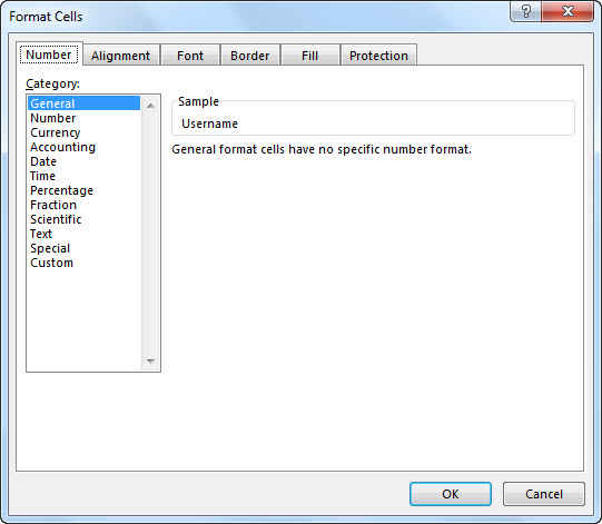
#10–Open “Format Cells” Dialog Box
The “format cells” dialog box helps format a cell or a cell range of Excel. To open this box manually, select a cell and right-click the same. Thereafter, choose the “format cells” option from the context menu.
The shortcut “Ctrl+1” (press together) opens the “format cells” dialog box.

Example
We want to open the “format cells” dialog box in an Excel worksheet with the help of the shortcut.
Step 1: In the worksheet, press “Ctrl+1” together.
Step 2: The “format cells” dialog box appears, as shown in the following image.
#11–Adjust Column Width
To adjust the width of a column, one needs to double-click the column edge. This task can also be done with the help of a shortcut.
The excel shortcut “Alt+O+C+A” (press one by one) adjusts the width of the selected column.

Example
The left side of the following image shows the usernames in column A. Since the width of this column has not been adjusted, some entries are exceeding its right-side border.
We want to adjust the width of column A with the help of the shortcut keys.
Step 1: Select the column (column A) whose width has to be adjusted.
Step 2: Press the shortcut keys “Alt+O+C+A” one by one.
Step 3: The column width is adjusted, as shown by the right side of the following image. Hence, all entries fit in column A.

#12–Repeat the Last Task
In Excel, one may need to repeat the last task or action performed. This task can be formatting, inserting a new row or column, deleting an existing row or column, and so on.
The shortcut “F4” repeats the last task, if possible.

#13–Insert Line Breaks in a Cell
While typing in a cell, there may be a need to insert a line break. The line break helps add spacing between the sentences of a cell. Once a line break is added, the user can begin a new sentence in the same cell.
The excel shortcut “Alt+Enter” (press together) inserts a line break within a cell.

Example
The following image shows a question in cell A1. We want to insert a line break in order to type a new sentence within the same cell A1. Use the shortcut for the same.
Step 1: Double-click the cell (cell A1) within which a line break is to be inserted.
Step 2: Click at the place (after the two question marks) where the line break is to be inserted.
Step 3: Press the keys “Alt+Enter” together. The line break appears, as shown in the following image. Hence, after the spacing has been inserted, the user can begin a new sentence in cell A1.
#14–Move Between Different Workbooks
To switch between various windows, the shortcut “Alt+tab” is used. However, often while working, one needs to move from one workbook to another.
The excel shortcut “Ctrl+tab” (press together) helps switch between the open workbooks.

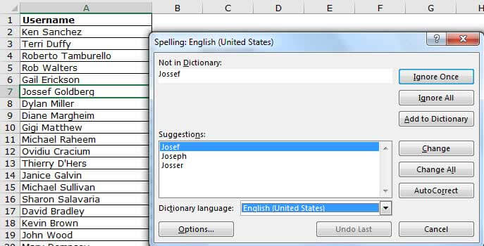
#15–Spell-Check
Prior to submitting an Excel worksheet to seniors at the workplace, it is essential to do a quick spell-check. This lets the user know the mistakes and the corrections that should be followed presently and in the future.
The excel shortcut “F7” helps perform a spell-check of the currently active worksheet.

Example
The following image shows the usernames in column A. We want to run a spell-check on this worksheet with the help of the shortcut.
Step 1: Press the shortcut “F7.”
Step 2: The “spelling” dialog box appears, as shown in the following image. Hence, the spellings of column A can be corrected by matching them against the suggestions.
#16–Move Between Worksheet and Excel VBA Editor
While working with macros, one needs to move between the VBA editor and the Excel worksheet.
The excel shortcut “Alt+F11” helps switch between the VBA editor and the worksheet.

#17–Select a Cell Range
Selecting the cell ranges of Excel can be a time-consuming task, if done manually.
The excel shortcut “Ctrl+Shift+arrow keys” selects the cell ranges of Excel.
Note: The selection of cells, in the same row or column as the currently active cell, is carried out till the last non-blank cell. However, if the following cell (in the same row or column as the currently active cell) is blank, the selection is carried out till the next non-blank cell.

Example
The following image shows the usernames, passwords, designations, titles, and first names in columns A, B, C, D, and E respectively. We want to select the range A1:E100 with the help of the shortcut.
Step 1: Select cell A1. Press the keys “Ctrl+Shift+right arrow” to select till cell E1.
Step 2: Press the keys “Ctrl+Shift+down arrow” to select till cell E100.
Step 3: The range A1:E100 is selected, as shown in the following image.
#18–Select the Last Non-Blank Cell of a Row or Column
Beginning from cell A1, one may need to go to the last cell of column A. This requires manual scrolling, which is a difficult task, particularly when working with large datasets.
The excel shortcut “Ctrl+down arrow” (press together) helps the user go to the last non-blank cell of the current column (column of the active cell).

The excel shortcut “Ctrl+right arrow” (press together) helps the user go to the last non-blank cell of the current row (row of the active cell).

Note: In case the cell immediately following the active cell is blank, the next non-blank cell is selected.
Example
The following table shows the usernames and passwords in columns A and B respectively. We want to go to the cell A100, which is the last non-blank cell of column A. Use the shortcut keys.
Step 1: Select cell A1. Press the keys “Ctrl+down arrow” together.
Step 2: The last cell (A100) of the dataset is selected, as shown in the following image.
#19–Delete the Active Sheet
To delete a sheet manually, one can right-click the sheet name and select “delete.” Alternatively, the shortcut helps do the same quickly.
The excel shortcut “Alt+E+L” (press one by one) deletes the currently active sheet.
Once the given shortcut is pressed, a message appears stating that the data of the worksheet will be permanently deleted. Click “delete” to delete the sheet, otherwise press “cancel.”

#20–Insert a New Sheet
Often, new sheets are required to be added to the workbook. It is possible to insert a new sheet with a single click.
The excel shortcut “Shift+F11” (press together) inserts a new sheet in the current workbook.

The excel shortcut “F11” inserts a chart sheet in which a chart can be created by selecting a data range.

Frequently Asked Questions
1. What are Excel shortcuts and how to use them?
An Excel shortcut helps perform a manual task in a faster way. With the application of shortcuts, the user saves time and improves the productivity. This saved time can be used for focusing on other projects of a job role.
The list of Excel shortcuts is a large one. There are shortcuts for entering, formatting, deleting, and selecting data. So, it is not possible to learn all the shortcuts. However, knowing the regularly used ones is essential.
To use an Excel shortcut, press the particular keys on the keyboard. But, prior to using it, one must know whether to press the keys simultaneously or one by one. This is because each shortcut works in a specific way.
2. What are the basic Excel shortcuts and how to learn them?
The basic Excel shortcuts are listed as follows:
Ctrl+S: It saves a workbook.
Ctrl+A: It selects the entire worksheet.
Ctrl+B: It makes the content of the selected cells bold.
Ctrl+C: It copies the selected cell.
Ctrl+I: It italicizes the content of the selected cell.
Ctrl+P: It opens the “print” dialog box.
Ctrl+X: It cuts the content of the selected cell.
Ctrl+V: It pastes in the currently selected cell.
Ctrl+Z: It undoes the last action.
Excel shortcuts can be learned with regular usage and practice. The more you practice working on Excel, the more habitual you will become. In this way, you can learn gradually.
Note: The keys of all the preceding shortcuts should be pressed simultaneously.
3. How to work with Excel formulas by way of shortcuts?
The “tab” key is an important shortcut used for auto-completing the name of the function. For instance, to enter the CONCATENATE function in a cell, type “=CON” and press the “tab” key. The CONCATENATE function is automatically selected.
With the “F4” key, one can toggle between the relative, absolute, and mixed references. Double-click the formula cell and press “F4” to change the type of reference.
Likewise, different keyboard keys have different functions. By applying shortcuts to Excel formulas, one can simplify working with calculations.
Recommended Articles
This has been a guide to the top 20 keyboard shortcuts in Excel. Here we discuss the working of keyboard shortcuts and how to use these Excel shortcuts to save your time. You may learn more about Excel from the following articles-