Data Table in Excel - Examples, Types, How to Create/Use?

What is Data Table in Excel?

A Data Table in Excel helps study the different outputs obtained by changing one or two inputs of a formula. A data table does not allow changing more than two inputs of a formula. However, these two inputs can have as many possible values (to be experimented) as one wants. Excel Data tables, along with Scenarios and Goal Seek are parts of the What-If Analysis tools.

Download FREE Data Table Excel Template and Follow Along!

Download Excel Template

For example, an organization may want to study how changes in the cash possessed impact its working capital. A data table will help the organization know the optimum level of cash (from the specified possible values) to be held to meet its short-term obligations.

The purpose of creating data tables in Excel is to analyze the variation in outputs resulting from a change in the inputs. Moreover, one can have all the outputs in a single table which eases interpretation and allows quick sharing with other users.

Types of Data Tables in Excel

The kinds of data tables in Excel are specified as follows:

One-variable data table
Two-variable data table

Let us discuss each type of data table one by one with the help of examples.

Note: A data table is different from a regular Excel table. The former shows the various combinations of inputs and outputs. These outputs are calculated by considering the source dataset as the base. In contrast, an Excel table shows related data that is grouped in one place.

One-Variable Data Table in Excel

A one-variable data table is created to study how a change in one input of the formula causes a change in the output. A one-variable data table in excel can be either row-oriented or column-oriented. This implies that all the possible values that an input can assume are listed in either a single row (row-oriented) or a single column (column-oriented) of Excel.

Example #1

There are two images titled “image 1” and “image 2.” The following information is given:

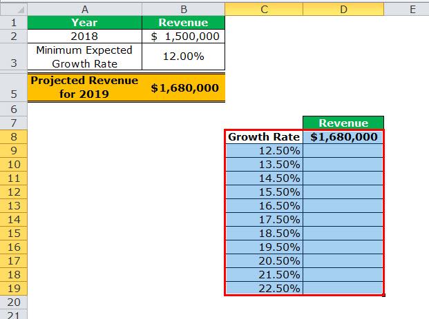
Image 1 shows an organization’s revenue (in $) for 2018 in cell B2. The minimum growth rate expected is given as 12% in cell B3. The projected revenue (in $ in cell B5) for 2019 has been calculated by using the formula “=B2+(B2*B3).”
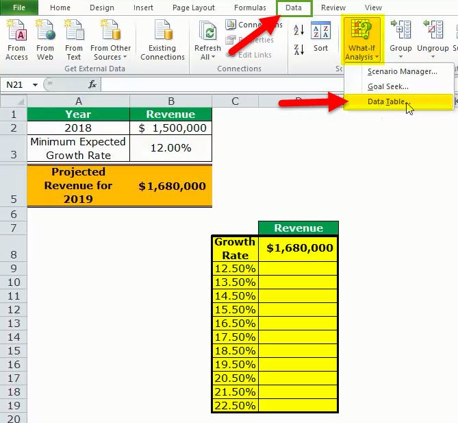
Image 2 shows the possible values (in column C) that the growth rate can assume. The value of cell D8 has been explained in steps 1 and 2 (given further in this example).

We want to perform the following tasks:

Calculate the projected revenues (in column D) according to the different growth rates (in column C) given in image 2.
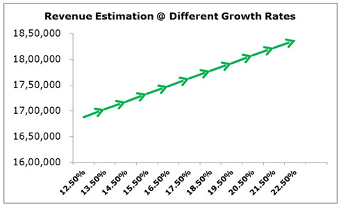
Create a “line with markers” chart showing the growth rates on the x-axis and the projected revenues on the y-axis. Replace the markers of the chart with arrows.

Use a one-variable data table of Excel. Interpret the data table thus created.

Image 1

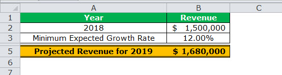
Image 2

The steps for performing the given tasks by using a one-variable data table are listed as follows:

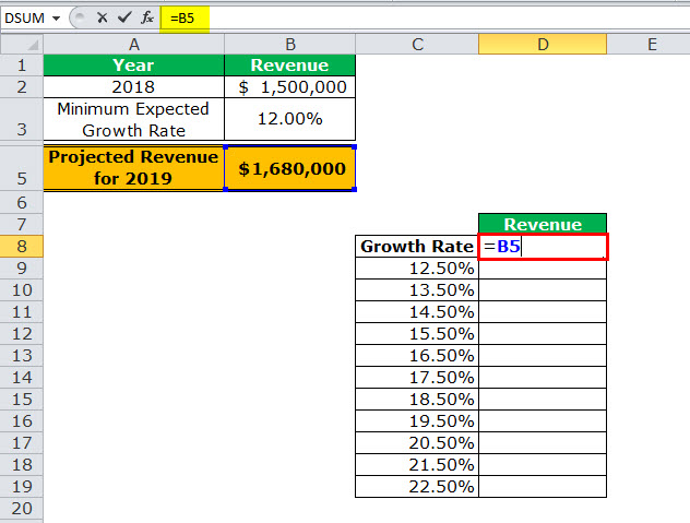
Enter the data of the two images in Excel. In cell D8, type “equal to” (=) followed by the reference B5. This links cell D8 to cell B5.
The linking of the two cells is shown in the following image.Since all the growth rates have been entered vertically (C9:C19), our data table is said to be column-oriented. The entire range C8:D19 is our one-variable data table. We are creating a one-variable data table as the change in outputs will be observed against a change in one input, i.e., the growth rate.Note:Notice that either the formula “=B2+(B2*B3)” could be typed directly in cell D8 or cell D8 can be linked to cell B5. We have chosen to link the two cells.The linking of cell D8 to cell B5 ensures that any updates in the formula of the latter are automatically reflected in the range D9:D19 of the data table. For instance, if the formula of cell B5 is multiplied by 2 [like =B2+(B2*B3)*2], all the outputs obtained in the range D9:D19 are automatically multiplied by 2.Had we not linked cells D8 and B5, any changes to the formula of cell B5 would not have changed the value in cell D8. Consequently, the outputs in the range D9:D19 would not have been updated automatically.
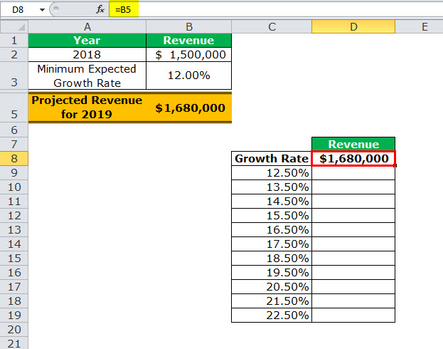
Press the “Enter” key. Cell D8 shows the value of cell B5, as shown in the following image.
Notice that if one manually enters the value (1680000) in cell D8, the data table will not work. Moreover, one should always type the formula [=B2+(B2*B3)] or link the cell that is one row above and one column to the right of the possible input values (C9:C19). This is the reason we chose to link cell D8 to cell B5.Note:If the data table is row-oriented, type the formula or link the cell that is one column to the left and one cell below the first possible input value. For instance, had the possible input values been in the range F2:P2, we would have entered the formula or linked cell E3 to cell B5.
Select the range of the data table. This selection should include the linked cell (D8), the possible input values (C9:C19), and the empty cells for outputs (D9:D19). Hence, we have selected the range C8:D19, as shown in the following image.
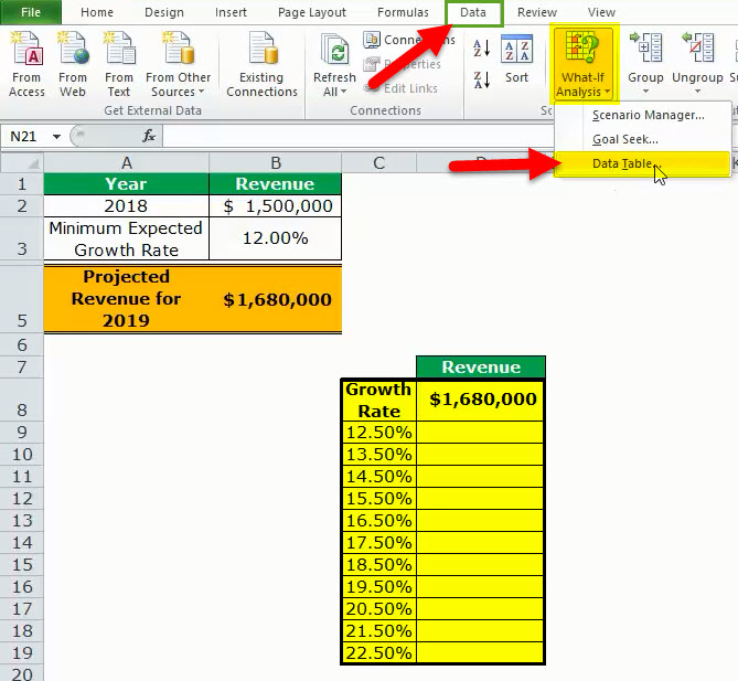
From the Data tab, click the “what-if analysis” drop-down (in the “data tools” or “forecast” group). Select the option “data table.” This option is shown in the following image.
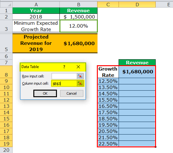
The “data table” dialog box opens, as shown in the following image. In the box of “column input cell,” select cell B3, which contains the minimum expected growth rate. As a result, the reference $B$3 appears in this box. Leave the box of “row input cell” blank.
By giving the reference to cell B3 in the “column input cell,” we are telling Excel that at the growth rate of 12%, the projected revenue is $1,680,000. So, with this data table, Excel is being asked the projected revenue when the growth rates vary from 12.5% to 22.5%.Note 1:A “row input cell” or “column input cell” is a reference to a cell that contains the input. This is the input that can assume the different possible values. Moreover, this input must necessarily be used in the formula whose outputs are to be studied.In a one-variable data table, either the “row input cell” or the “column input cell” is specified depending on whether the data table is row-oriented or column-oriented.Note 2:In a one-variable data table, Excel uses either the formula “=TABLE(row_input_cell,)” or “=TABLE(,column_input_cell)” to calculate the different outputs. The former formula is used when the possible input values are in a row, while the latter is used when the possible input values are in a column.To view the TABLE formula, select any of the output cells and check the formula bar. In this example, the formula “=TABLE(,B3)” is used to calculate the outputs.Further, Excel uses these TABLE formulas as array formulas. However, these formulas cannot be edited manually, unlike the regular array formulas. But, one can delete all the output cells containing the TABLE formulas.
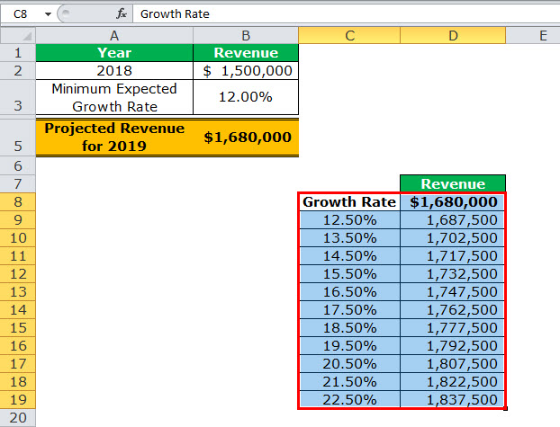
Click “Ok” in the “data table” window. The range D9:D19 of the data table has been filled with values. The different outputs are shown in the following image.
Interpretation of the one-variable data table:By looking at the data table in the preceding image, one can say that when the growth rate is 12.5%, the projected revenue is $1,687,500. Likewise, when the growth rate is 13.5%, the projected revenue is $1,702,500. Hence, the larger the growth rate, the more the increase in the projected revenue.The projected revenue is at its maximum ($1,837,500) when the growth rate is at its highest (22.5%). So, the organization can study the variation in outputs when a single input (growth rate) changes.Note:For more examples related to the one-variable data table of Excel, refer to the hyperlink given before step 1.
To create a “line with markers” chart that displays the growth rates on the x-axis and the projected revenues on the y-axis, follow the listed steps:
a.Select the range D9:D19 and click the Insert tab on the Excel ribbon.b.Click the “insert line or area chart” icon from the “charts” group. Select the “line with markers” chart under the 2-D line charts. A “line with markers” chart appears, which displays the projected revenues on the y-axis.c.Click anywhere on the chart. The “chart tools” menu becomes visible. This menu consists of the Design and Format tabs.d.Click the Design tab of the “chart tools” menu. Choose “select data” from the “data” group. The “select data source” window opens.e.Click “edit” under “horizontal (category) axis labels.” The “axis labels” window opens.f.Select the range C9:C19 in the “axis label range” box. Click “Ok.” Click “Ok” again in the “select data source” window.The “line with markers” chart is created whose x-axis and y-axis look the way they are shown in the image of step 8.
To replace the default markers of the chart with arrows, follow the listed steps:
a.Select the markers of the chart and right-click them. Choose the “format data series” option from the context menu. The “format data series” pane opens.b.Click the “fill u0026 line” tab. Expand the “line” tab. In “end arrow type,” select any of the arrows. We have chosen “open arrow.”c.Select “marker” and expand the “marker options.” Choose the option “none.”d.Close the “format data series” pane.The “line with markers” chart looks the way it is displayed in the following image. Notice that since the chart shows the projected revenues, we have titled it accordingly.

Two-Variable Data Table in Excel

A two-variable data table in excel helps study how changes in two inputs of a formula cause a change in the output. In a two-variable data table, there are two ranges of possible values for the two inputs. From these two ranges, one range is in a row and the other is in a column of Excel.

Example #2

There are three images titled “image 1,” “image 2,” and “image 3.” The following information is given:

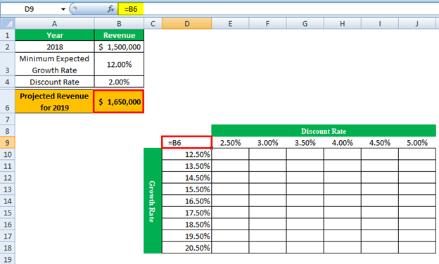
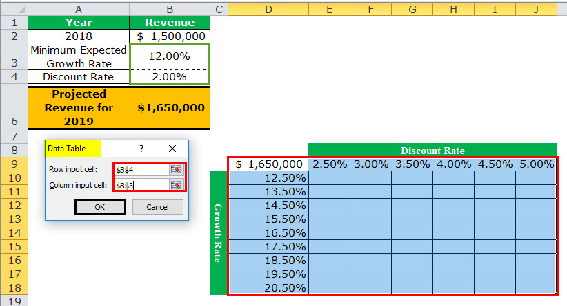
Image 1 shows an organization’s revenue (in $ in 2018) and the minimum growth rate in cells B2 and B3 respectively. Both these figures are the same as that of the previous example. Additionally, the organization gives a 2% discount (in cell B4) to its customers. This is given to boost sales.
Image 2 shows how the projected revenue (in $ in cell B6) for 2019 has been calculated. The formula “=B2+(B2*B3)-(B2*B4)” is used for this purpose. The amount obtained ($1,650,000) is the projected revenue after the discount.
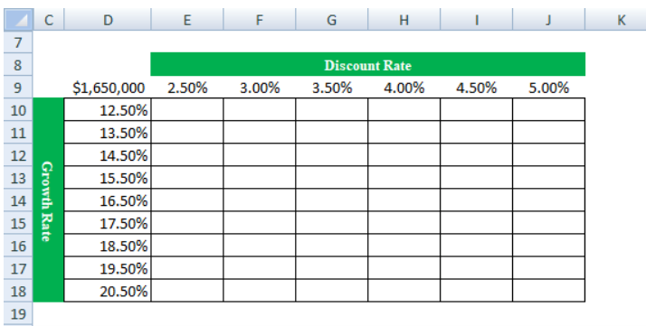
Image 3 shows the different values in row 9 that the discount rate can assume. The possible values that the growth rate can assume are given in column D. The value of cell D9 has been explained in steps 1 and 2 (given further in this example).

Calculate the projected revenues (in E10:J18) according to the various discount rates (in row 9) and growth rates (in column D). Use a two-variable data table of Excel. Interpret the data table thus created.

Image 1

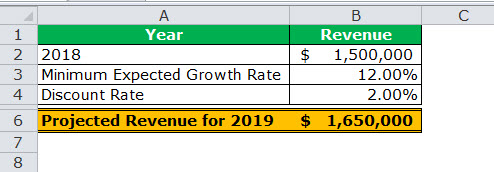
Image 2

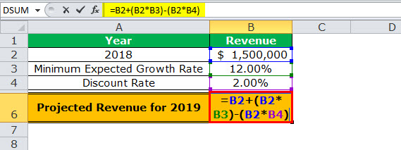
Image 3

The steps for creating a two-variable data table are listed as follows:

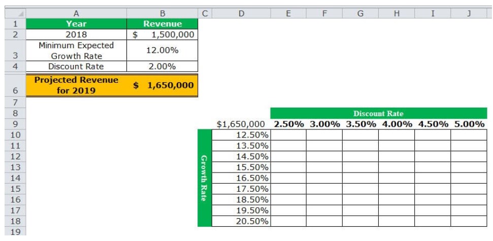
Step 1: Enter the data of the preceding images in Excel. In cell D9, type the “equal to” operator followed by the reference B6.

This time we have chosen to link cell D9 to cell B6. Alternatively, we could have also entered the formula [=B2+(B2*B3)-(B2*B4)] in cell D9. This is because, in a two-variable data table, one should type the formula or link the cell that is one column to the left of the first horizontal input value (2.5%). At the same time, this cell should be one row above the first vertical input value (12.5%).

The linking of cells ensures that any changes to the formula of cell B6 are reflected in the value of cell D9. Further, any change in the value of cell D9 will update the outputs (in E10:J18) automatically.

Note: Please ignore the differences in font, colors, and alignment across the images of this example. These differences may be due to the different versions of Excel being used to create the images.

Step 2: Press the “Enter” key. Cell D9 shows the value of cell B6, which is 1,650,000. This is shown in the following image.

The entire range D9:J18 is our two-variable data table. Notice that the excel data table shows the possible discount rates horizontally (in bold in row 9) and the possible growth rates vertically (in column D). This time the variation in outputs resulting from changes in both these inputs (discount rate and growth rate) need to be studied.

Note: If the value is entered manually in cell D9, the excel data table will not work.

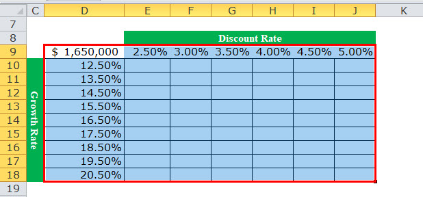
Step 3: Select the range D9:J18. Note that the selection should include the linked cell (D9), possible discount rates (E9:J9), possible growth rates (D10:D18), and the empty cells for the outputs (E10:J18).

The selection is shown in the following image.

Step 4: Click the “what-if analysis” drop-down (in the “data tools” or “forecast” group) of the Data tab. Select the option “data table.”

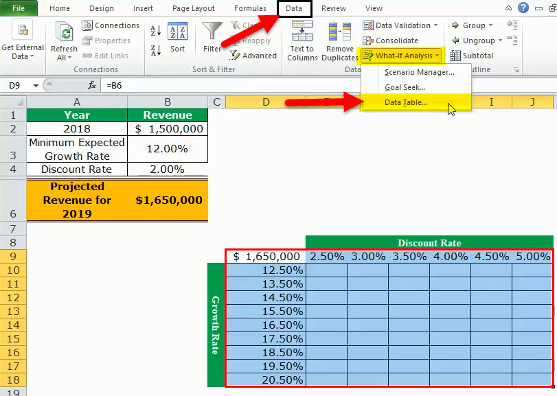
Step 5: The “data table” window opens, as shown in the following image. In the box of “row input cell,” select cell B4. In the box of “column input cell,” select cell B3. The absolute references to cells B4 and B3 appear in the two boxes.

Cells B4 and B3 contain the minimum expected growth rate and the discount rate of the source dataset.

By making these selections, Excel is told that at a discount rate of 2% and a growth rate of 12%, the projected revenue is $1,650,000. Therefore, our two-variable data table instructs Excel to calculate the projected revenues when the discount rates and growth rates vary from 2.5% to 5% and 12.5% to 20.5% respectively.

Note: In a two-variable data table, both the “row input cell” and “column input cell” are specified, unlike a one-variable data table where one has to specify either of the two inputs.

Further a two-variable data table uses the formula “=TABLE(row_input_cell,column_input_cell)” to calculate the outputs. So, in this example, the formula “=TABLE(B4,B3)” has been used for the calculations. This formula is visible in the formula bar when an output cell is selected.

For the meaning of the “row input cell” and the “column input cell,” refer to “note 1” under step 5 of example #1.

Step 6: Click “Ok” in the “data table” window. The outputs appear in the range E10:J18, as shown in the following image.

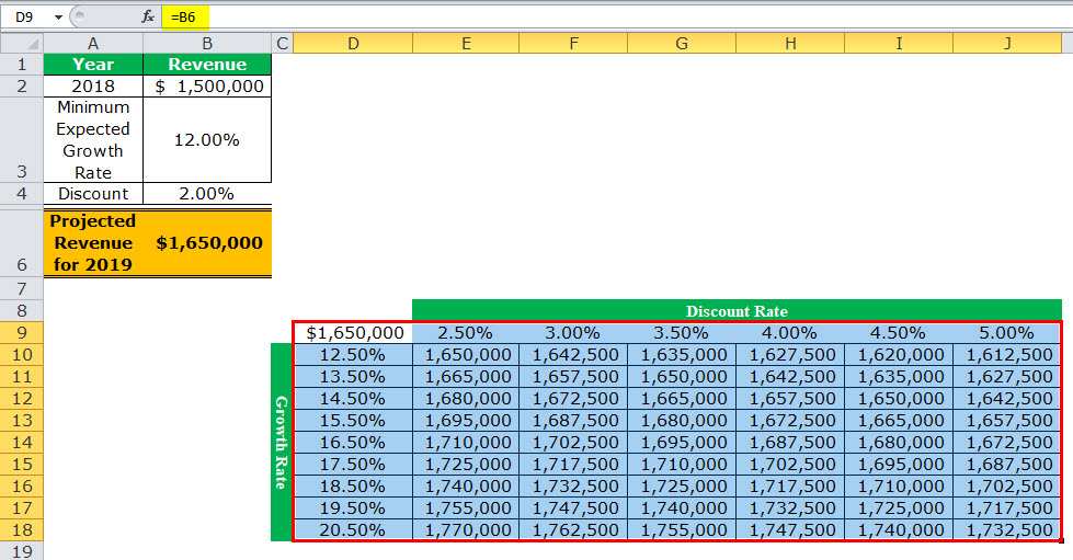
Interpretation of the two-variable data table: When the discount rate is 2.5% and the growth rate is 12.5%, the organization’s projected revenue is $1,650,000 (in cell E10). Notice that this figure is the same as that of cell B6. However, the value in cell B6 takes into account 2% and 12% as the discount rate and growth rate respectively.

Notice that the numbers of cells E10 and B6 match those of cells G11 and I12. This implies that when the discount rate and growth rate are increased in the same proportion (like by 0.5%, 1.5% or 2.5%), the resulting value is the same as the output of the source dataset (in cell B6). Cells E10, G11, and I12 reflect 0.5%, 1.5%, and 2.5% increase in the two rates.

Likewise, had we increased both the discount and growth rates by 1%, the resulting value would have again been $1,650,000. In this case, the discount rate and growth rate would have been 3% and 13% respectively.

By obtaining the projected revenues in the range E10:J18, the organization can sell at an optimum discount rate and, at the same time, target an attainable growth rate. Hence, the organization can choose the most suitable combination of the two rates.

Note: For more examples related to the two-variable data table of Excel, click the hyperlink given before step 1 of this example.

The Key Points Governing Data Tables in Excel

The important points related to data tables of Excel are listed as follows:

It helps select those input values that fit the business in the best possible manner.
It facilitates the comparison of the different outputs as all the results are consolidated in one place.
It presents the results in a tabular format that can neither be edited nor undone with the shortcut “Ctrl+Z.” The outputs can only be deleted by selecting them and pressing the “Delete” key.
It uses the TABLE array formulas to calculate the outputs. The “row input cell” and the “column input cell” must be selected carefully to get accurate results. Moreover, the input cell or cells must be on the same worksheet as the data table.
It need not be refreshed, unlike a pivot table. A change in the values or the formula of the source dataset causes the excel data table to update automatically.

Frequently Asked Questions (FAQs)

1. Define a data table and suggest when it should be used in Excel.

A data table helps analyze how a change in one or two inputs of a formula causes a change in the output. The resulting outputs are arranged in a tabular format, making them easy to compare and interpret.
A data table of Excel should be used in the following situations:

When the outputs resulting from a change in one or two inputs need to be studied
When the most optimum input value or values need to be chosen
When all the combinations of inputs and outputs need to be explored in one glance

2. How to create a data table in Excel?

The steps to create a data table in Excel are listed as follows:

a. Enter the source dataset in an Excel worksheet. Use one or two inputs to calculate an output.
b. Arrange the possible values, which an input can assume, in a row and/or column.
c. Link one cell of the data table to the output cell of the source dataset. Alternatively, in a cell of the data table, enter the formula whose outputs need to be studied.
d. Select the data table. The selection should include the linked cell (or the formula cell of the data table), the possible input values, and the empty cells for outputs.
e. Select the “data table” option from the “what-if analysis” drop-down of the Data tab. The “data table” window opens.
f. Enter either the “row input cell” or “column input cell” if the impact of changing one input is to be studied. To study the impact of changing two inputs, enter both “row input cell” and “column input cell.”
g. Click “Ok” in the “data table” window.

A one-variable or two-variable data table is created depending on the execution of steps “a,” “b,” and “f.”

Note: For more details on creating a data table in Excel, refer to the examples of this article.

3. How does a data table work in Excel?

A data table works on the policy “what will be the result if one or two inputs of a formula are changed?” One cell of the data table is linked to the source dataset. In this way, Excel is told how the inputs are to be used in calculating the output.

Next, as the possible input values are supplied, Excel is asked to calculate the outputs using the same formula as that of the source dataset. The resulting table shows the different mixes of inputs and outputs, thereby assisting the user in decision-making.