Tables in Excel

Tables in Excel helps group related data into one or more rows and/or columns. Once a table is created, Excel assigns a unique name to the columns and the table itself. Such names are used as structured references, which make it easy to apply Excel formulas. Therefore, tables eliminate the need to create named ranges in Excel.

For example, the following image shows a usual data range on the left side and an Excel table on the right side. Notice the alternately colored excel rows and structured references (in cell J2) of the latter.

The purpose of creating tables is to make the data manageable, organized, and fit for analysis. Apart from structured references, tables offer several benefits like quick sorting and filtering, automatic expansion, easy formatting, readable formulas, and so on. Tables are extremely helpful when working with large databases.

A table can be customized by changing its name and/or the default color (or table style). Let us learn how this is done.

#1–Change the Name of the Table

When a table is created, Excel assigns a default name like “table1,” “table2,” etc., depending on whether it is the first or the second table of the current workbook.

Working with such default names may become confusing, especially when there are lots of tables. So, the solution is to assign unique names to each table.

The steps for changing the name of the Excel table are listed as follows:

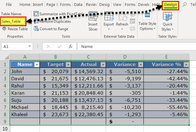
Step 1: Select the entire table. Once selected, the Design tab appears on the Excel ribbon. This tab is shown within a red box in the following image.

Note: In place of the entire table, even if a single cell is selected, the Design tab will become visible.

Step 2: In the Design tab, perform the following tasks:

• Click inside the box under “table name.” This box is displayed in the “properties” group at the leftmost side of the ribbon.
• Enter the desired name in this box.
• Press the “Enter” key.

Our table has been named “Sales_Table.” This is shown in the following image.

Rules Governing the Table Names

While naming a table, the following points should be considered:

• The name should always begin with a letter, a backslash () or an underscore (_).
• The name cannot be the single letter “r” (or “R”) or “c” (or “C”).
• The name should not consist of any spaces. Instead, one can use an underscore (_) or a period (.) to separate the words.
• The name can contain numbers, but cell references should be avoided.
• The name can contain a maximum of 255 characters.
• The name of the table should be unique. In case of a duplicate name, a message will be displayed saying that a unique name should be chosen.

Note: A name is said to be duplicate if two tables within the same workbook have the same names. Further, Excel does not distinguish between the uppercase and lowercase letters in the name of a table. So, the names “abc” or “ABC” are considered the same by Excel.

#2–Change the Color of the Table

When a table is created, Excel assigns it a default color. To change the color of the table, its style needs to be changed. Excel displays a list of different table styles from which one can choose the desired option.

The steps to change the color (or style) of a table are listed as follows:

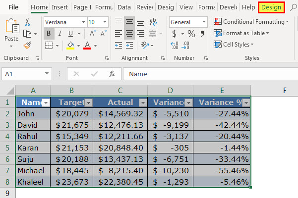
Step 1: Select either a cell of the table or the entire table. We have selected the latter. The Design tab becomes visible, as shown in the following image.

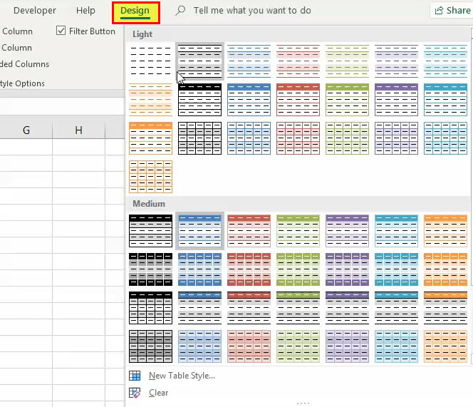
Step 2: Choose the desired color (or style) from the “table styles” group of the Design tab. To expand the list of table styles, click the “more” button displayed at the bottom right side. One can also click “new table style” to view more styles.

The following image shows the expanded list of table styles. Once the desired style is chosen, it will be applied to the entire table.

Note: The default table style of the workbook can be changed by the user. For making this change, perform the listed steps:

• Select the desired table style from the list of table styles.
• Right-click the selected table style and choose “set as default” from the context menu.

Let us discuss eight advantages of creating tables in Excel.

#1–Creates Structured References Automatically

An Excel table uses structured references for referencing one or more cells. This is in contrast with the direct cell addresses used in a normal data range. A structured reference is a combination of table and column names that are used in Excel formulas.

The major benefits of using structured references are listed as follows:

1. They automatically update when new entries are added or deleted from the table.
2. They are automatically created when one or more cells of the table are selected.
3. They can be used both within and outside the table, thus making it easy to locate tables in a workbook.
4. They are used to autofill the calculated columns. A calculated column is an additional column added to the existing Excel table. It uses a single formula that expands on its own in the remaining part of the column. This implies that when a formula is entered in one cell of a calculated column, it need not be dragged to the remaining cells of the column. Rather, the formula is automatically entered in all cells (called autofill), unlike a usual data range which requires one to drag the fill handle.

Example of point “d”: The range A2:B7 is an Excel table containing random numbers. To create column C as a calculated column, enter the SUM formula in cell C3, which adds the numbers of cells A3 and B3. Use structured references in this formula. Once the formula is entered, press the “Enter” key. The outcomes are stated as follows:

• The table (A2:B7) automatically expands to include column C.
• The range C4:C7 is automatically filled with the totals of each row of the table. 

The preceding results will be obtained with both structured and regular references. This is because autofilling is a feature of Excel tables. However, with structured references, it is easy to read and understand the formula.

Note that if the user makes a change to the formula of the calculated column, the change is automatically replicated in the entire column.

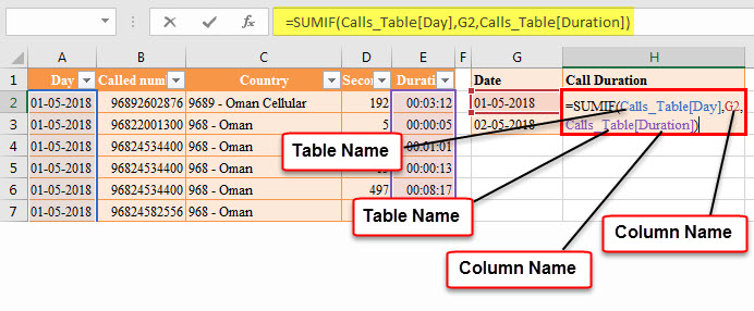
Example of structured references: In the following image, structured references have been used in the SUMIF formula. The “Calls_Table” is the name of the Excel table. “Day” and “duration” are the names of columns A and E respectively. The cell G2 is a direct cell reference.

Note: In the following image, the black line pointing to cell G2 has been incorrectly placed. It should have pointed to “day,” which is the name of column A. So, please ignore the misplacement.

#2–Is Dynamic in Nature

Any new insertions to the cells below or to the right of the table are automatically included in the Excel table. This implies that the table expands to include such insertions. Likewise, the table contracts when one or more rows and/or columns are deleted from it. Due to automatic expansion and contraction, an Excel table is often considered a dynamic table.

Expansion implies that the style, formatting, and formulas of the table are automatically applied to the new entries as well. This eliminates the need to format and edit the formulas of individual cells. By default, the formatting stays uniform throughout an Excel table.

Note that the formulas of the table are adjustable as they take into account structured references. In contrast, the formulas of a normal data range do not adjust with insertions or deletions of entries.

Note: To undo table expansion, press the keys “Ctrl+Z” together.

#3–Makes it Easy to Work With PivotTables

It is advised to create a PivotTable from an Excel table. The major reasons the source data should be an Excel table are listed as follows:

• A PivotTable automatically updates with any changes in the source table. Since Excel tables are dynamic, the data range of the PivotTable also becomes dynamic.
• A single cell of the source table can be selected prior to inserting a PivotTable. In contrast, when the source data is a usual data range, the entire range (or dataset) needs to be selected prior to inserting a PivotTable.

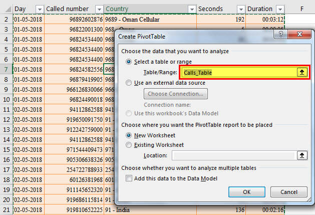
For instance, in the following image, a single cell of the source table has been selected before clicking the “PivotTable” option from the Excel Insert tab. Notice that in “table/range,” the name of the source table is reflected.

#4–Freezes Header Row Automatically

When one scrolls downwards in a worksheet, the table headers are visible at all times. This is because these headers are automatically fixed or frozen at their respective places.

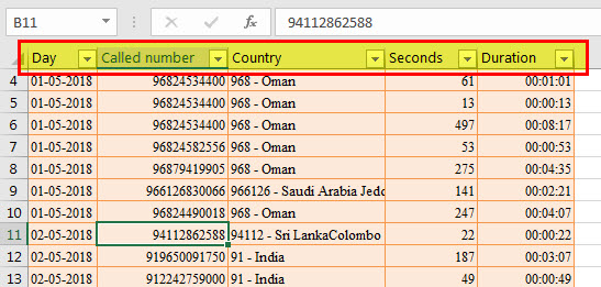
Fixed headers prevent the user from going back to the top row (row 1) again and again. Such frozen headers can be seen within a red rectangle in the following image.

Notice that the user has scrolled downwards such that rows 4 to 13 are visible along with the header row.

Note: To see the frozen header row, ensure that a cell of the table is selected before scrolling.

#5–Helps add a Total Row Containing Functions

An Excel table shows various functions in the total row. For displaying this row, perform the following steps:

• Select any cell of the Excel table. The Design tab appears on the Excel ribbon.
• From the Design tab, select the checkbox of “total row” displayed in the “table style options” group.

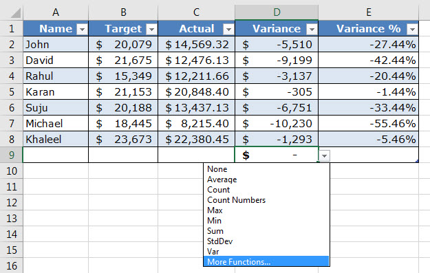
The total row is added immediately below the Excel table. Select any cell of this row to see a drop-down arrow on the right side. When this arrow is clicked, a list containing functions appears, as shown in the following image.

Once a function is selected from the list, the respective formula is automatically entered and the output is shown in a cell of the total row.

Notice that row 9 of the following image is the total row. Further, if a function is selected in cell D9, the corresponding output will also be displayed in this cell. The formula will be visible in the formula bar of the worksheet.

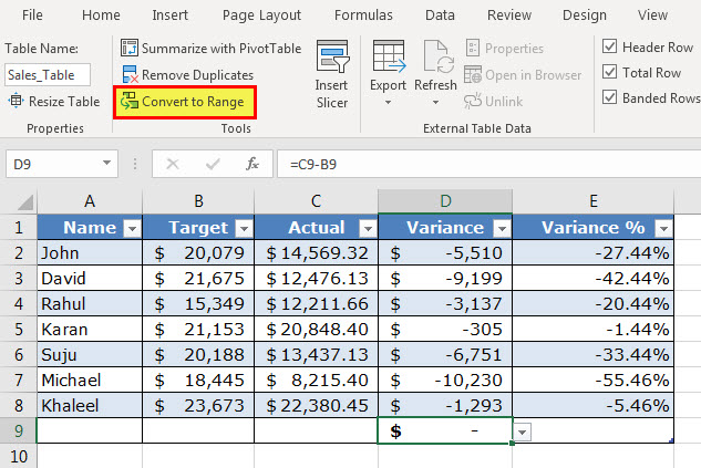
#6–Eases Restoring to Usual Data Range Without Losing the Table Style

An Excel table can be quickly converted to a usual data range. This serves as a benefit when the user requires only the table style and not the functionality of the table. For such conversion, follow either of the listed steps:

• Select any cell of the table. From the Design tab, click “convert to range” in the tools group.
• Select any cell of the table and right-click it. From the context menu, choose “table” followed by “convert to range.”

The “convert to range” feature of the first pointer is shown in the following image. Once an Excel table is converted to a usual data range, the existing structured references are replaced with the regular cell references. However, the data and formatting of the table are retained in the usual data range.

Note: The “convert to range” feature can be used only when the data to be converted is in the form of an Excel table.

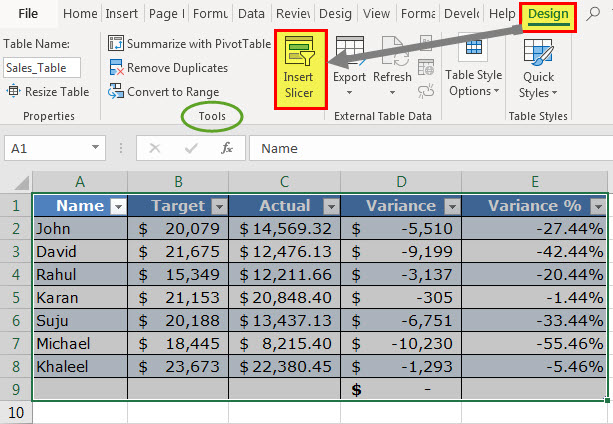
#7–Helps add Slicers for Filtering Data

A slicer helps filter the data of an Excel table. It displays buttons that can be selected or deselected to indicate whether an item is included or excluded from the filter.

Slicers are available in Excel 2013 and the newer Excel versions. The steps to add a slicer to a table are listed as follows:

1. Select either a cell within the table or the entire table.
2. From the Design tab, select “insert slicer” from the “tools” group.
3. The “insert slicer” dialog box opens. Next, select the checkboxes of the columns for which the slicer needs to be created.
4. Click “Ok.”

One can have a slicer for each column of the Excel table. Once slicers appear in the worksheet, they can be moved, resized, and formatted according to the requirement.

With a slicer, one can filter and view only particular items (or entries) of the table. To view multiple items of a column, press and hold the “Ctrl” key while selecting the items in the respective slicer.

The following image shows the “insert slicer” option of the Design tab.

Note 1: A slicer can also be added from the “filters” group of the Insert tab of Excel. Click “slicer” in this group and thereafter follow the steps “c” and “d” listed above.

Note 2: A slicer can be used only if the data is in the form of an Excel table.

#8–Assists in Creating Reports in Power BI

Excel tables serve as a source from which data is entered in the Power BI tool. Power BI is a business intelligence tool that helps convert unrelated sources of data into meaningful reports and dashboards. The process of creating reports works as follows:

• Create and upload Excel tables to Power BI. 
• Create a report in Power BI by adding visualizations.
• Share the report with other Power BI users or office colleagues.

Excel tables are a preferred data source in Power BI due to the following reasons:

• They allow quick access to the tabular format of the dataset.
• They help ease comparisons within a dataset.
• They can be easily edited and organized prior to being uploaded in Power BI.

The steps to turn off structured references in Excel are listed as follows:

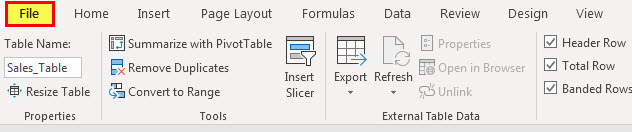
Step 1: Click the File tab of Excel. It is displayed within a red box in the following image.

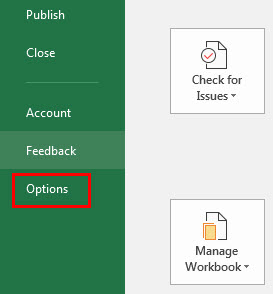
Step 2: Select “options” shown in the following image.

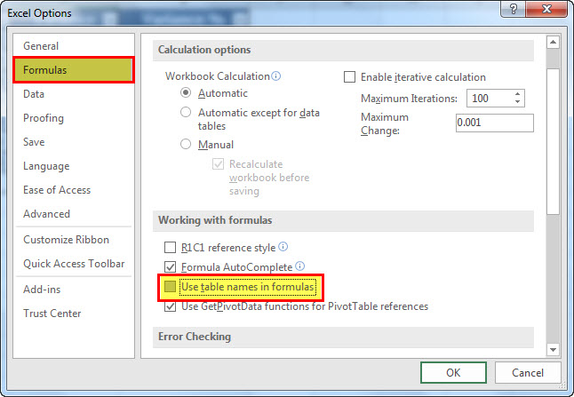
Step 3: The “Excel options” dialog box opens. Click “formulas” appearing on the left side of the window. Deselect the checkbox of “use table names in formulas.” This is shown in the following image.

Next, click “Ok.” The structured references will be turned off in Excel.

Note: By changing this setting, the structured references used in the existing formulas of the Excel table are not removed. However, the new formulas applied to the table will contain regular cell references instead of structured references. If regular cell references are required in existing formulas too, they will have to be edited manually.

Further, whether the structured references are turned on or off, the changed setting will be applied to all workbooks that the user is working on.

This has been a guide to tables in Excel. Here, we explain how to create/insert/customize Excel tables along with examples and advantages. You may also look at these useful functions of Excel–

• Delete Pivot Table Excel
• Refresh Pivot Table in Excel
• Data Table in Excel
• Excel Merge Tables