What is a Checklist in Excel?
A checklist is a checkbox in Excel used to represent whether a given task is completed. Normally, the value returned by the checklist is either true or false. But, we can improvise with the results. When the checklist is tick marked, the result is true, and when it is blank, the result is false. We can insert a checklist from the “Insert” option in the “Developer” tab.
For example, you must keep track of activities, tasks, or processes. Again, a checklist in Excel is the best option. It can help you maintain a record in the spreadsheet as you complete the job or items. Moreover, you may also view them to know when you have checked off everything.
In Excel, we can create a checklist template that keeps us updated with all the tasks needed for a particular project or event.
We all plan our tasks, events, etc. We usually memorize or note down somewhere to check the list of tasks that need to be completed or the list of completed jobs.
Planning for an event, marriage, or work includes many steps or projects at different time frames. Naturally, therefore, we need many tasks to be completed on time. However, remembering all those tasks is a list that is not a walk in the park; maintaining the Excel checklist is not easy on paper.
If you have experienced such problems, you can learn how to create checklists in Excel. This article will introduce you to the interactive Excel checklist template.
How to Create a Checklist in Excel Using CheckBoxes?
The most common way of creating an excel checklist template is using CheckBoxes in Excel. In our earlier article, we elaborated on using checkboxes. The checkboxes represent the selection and deselection visually.
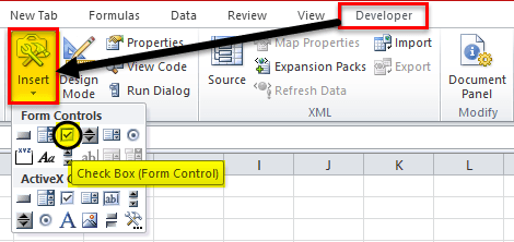
The checkbox is available under the “Developer” tab. If you cannot see the “Developer” tab, enable it. Once the “Developer” tab is enabled, you can see the checkbox below.
Examples
Examples #1
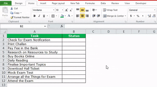
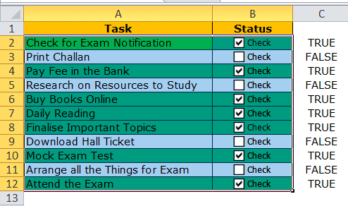
We will explain the simple Excel checklist template. Below are the tasks that need to be carried out before the exam.
| Task | Status |
|---|---|
| Check for Exam Notification | |
| Print Challan | |
| Pay Fee in the Bank | |
| Research on Resources to Study | |
| Buy Books Online | |
| Daily Reading | |
| Finalize Important Topics | |
| Download Hall Ticket | |
| Mock Exam Test | |
| Arrange all the Things for the Exam | |
| Attend the Exam |
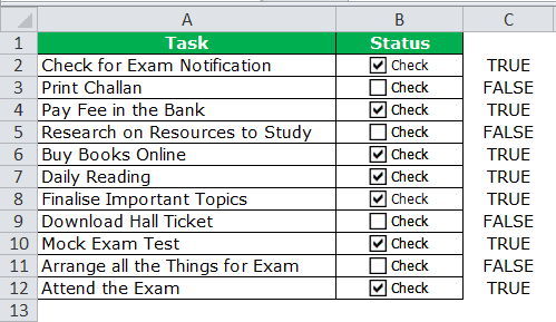
We will copy this list into Excel. Then, first, we will go to the “Developer” tab, select “CheckBox,” and draw in the B2 cell.
Now, we will drag the checkbox against all the task lists.
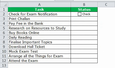
As a result, now we have the checkbox for all the tasks.
Next, we will right-click the first checkbox and select “Format Control” in Excel.
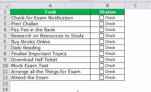
Under “Format Control,” we must go to “Control” and select “Checked,” and give cell reference to the C2 cell.
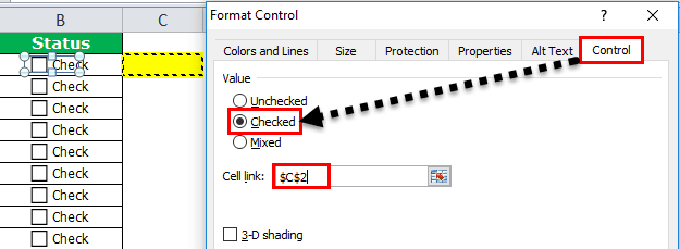
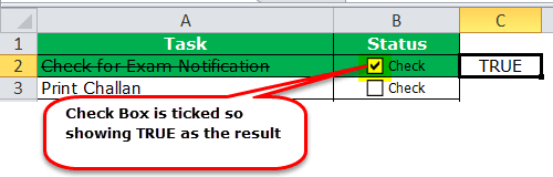
Now, this checkbox is linked to cell C2. So, if the checkbox is ticked, as a result, in C2, it will show “TRUE.” Else, it will display “FALSE” in cell C2.
Similarly, we will repeat the same task but keep changing the cell reference to the individual cell. So, for example, for the next checkbox, we will give the cell reference as C3, for the next, we will provide a cell reference as C4, and so on.
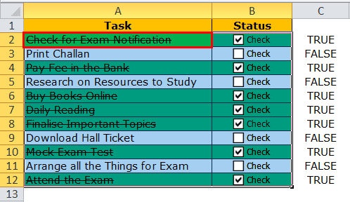
Finally, it will complete all our checkbox settings. It should look like the one below, as shown in the image.
We keep ticking the respective task boxes to update our task list template as the tasks are completed.
Example #2 – How to Make Your Checklist More Attractive?
The above checklist list template looks ordinary. However, we can make this a beauty by adding colors to it.
1. We must select all the tasks.
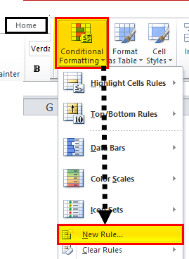
2. Then, we must go to the “Home” tab and select “Conditional Formatting,” then “New Rule.”
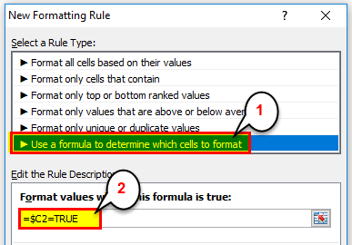
3. Under “New Rule,” we will mention the formula as =$C2= TRUE.
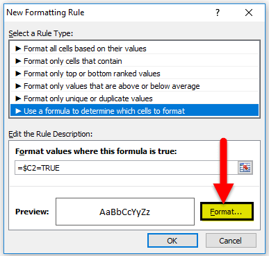
4. Now, we will click on “Format.”
5. Under “Format Cells,” we will go to “Fill” and select the color to highlight the completed task.
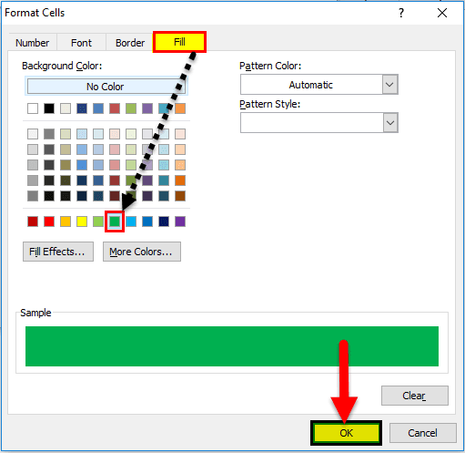
6. Lastly, we will click on “OK” to complete the procedure. If the checkbox is ticked, we will get a result as “TRUE” in column C, or we will get the result as “FALSE.”
“Conditional Formatting” looks for all the “TRUE” values. If any “TRUE” value is found in column C, it will highlight the Excel checklist area with green color.
Example #3 – Strikethrough all the Completed Excel Check List
We can make the report more beautiful by going one extra mile in conditional formatting. We can strikethrough all the completed checklist templates with conditional formatting.
In general perception, strikethrough means something which is already completed or over. So, we will apply the same logic here as well.
Step 1: First, we must select the checklist data range.
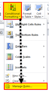
Step 2: Now, we need to go to “Conditional Formatting” and click “Manage Rules.”
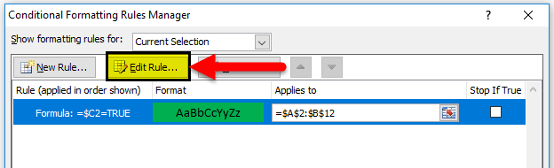
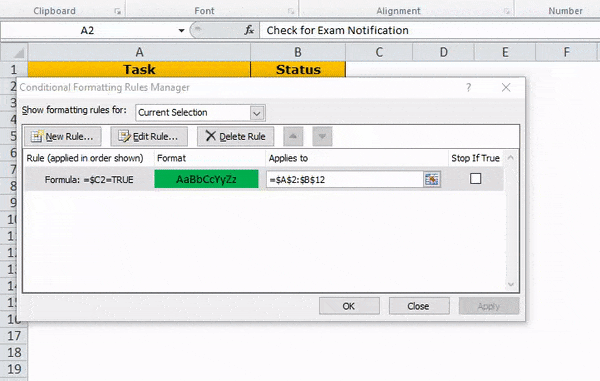
Step 3: We can see all the “Conditional Formatting” lists. Then, select the rule and click on “Edit Rule.”
Step 4: Now, we need to click on “Format,” choose “Font,” and select “Strikethrough.”
Step 5: Then, we will click on “OK.” As a result, all the tasks which are completed will be strikethrough.
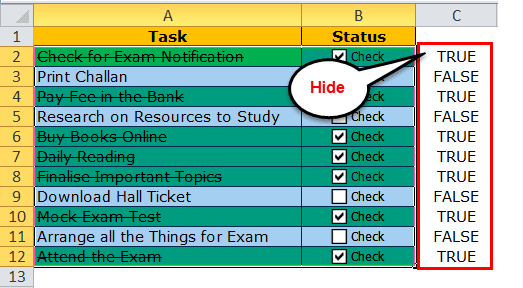
Step 6: We will hide column C to make the checklist template more beautiful.
Things to Remember about Checklist in Excel
- Choose light color under conditional formatting to highlight.
- Strikethrough will be the sign of something already completed.
- Instead of time-consuming checkboxes, we can create a dropdown list of completed and not completed.
Recommended Articles
This article is a guide to Checklist in Excel. We discuss how to create a checklist in Excel, along with Excel examples and downloadable Excel templates. You may also look at these useful functions in Excel: –