Name Manager in Excel | How to Create, Use & Manage Names in Excel?

Excel Name Manager

Named Ranges in excel formulas can be used as a substitute for cell references. Excel Name Manager is used to create, edit, delete and find other names in the Excel workbook.

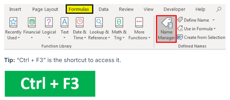
Download FREE Name Manager In Excel Template and Follow Along!

Download Excel Template

Excel “Name Manager” can be found in the “Formulas” tab.

Tip: “Ctrl + F3” is the shortcut to access it.

Usually, it is used to work with existing names. However, it also allows you to create a new name too.

How to Use Name Manager in Excel?

Please follow the below steps for using the Excel Name Manager.

First, we must go to the “Formulas” tab > “Defined Names” group, then click the “Name Manager.” Alternatively, we can press “Ctrl + F3” (the shortcut for Name Manager).
For a new named range, click on the “New” button.
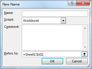
You may see the window below by clicking the “New” button.
Type in the name we want to give to the range and the cells it will refer to in the “Refers to” section.

Examples of Name Manager in Excel

We can use Name Manager to create, edit, delete and filter Excel names. Below, we will see one example of each, along with their explanations.

Example #1 – Creating, Editing & Deleting Named Range in Excel

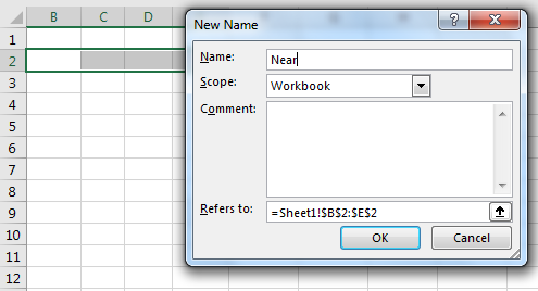
Let us suppose we want to refer to the cells in the range B2:E2 by the name “Near.” To do that, follow the below steps.

Go to the “Formulas” tab > “Defined Names” group, then click the “Name Manager.” Alternatively, we can press “Ctrl + F3” (the excel shortcut for Name Manager).

For a new named range, click on the “New” button.

Then in “Name,” write “Near,” and in “Refer to,” select B2: E2 and click “OK.”

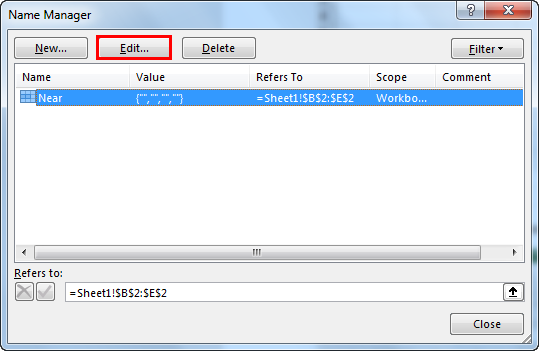
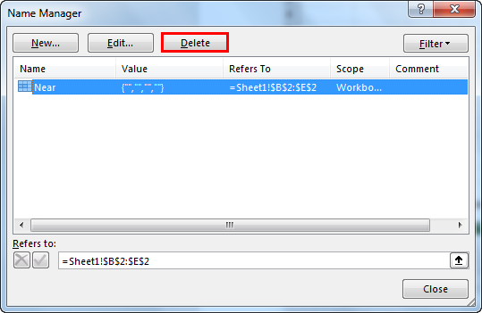
After this, we can see the name “Near” created when we click on the Excel “Name Manager.”

We can see the other options like “Edit” and “Delete.” Let us suppose we want to edit the cell reference. Then select the relevant named range (here “near”), click on “Edit,” and change the configuration.

Similarly, select the relevant named range for deleting and click on “Delete.”

If we want to delete multiple named ranges at once, we only need to select the relevant ones by pressing the “Ctrl” button. After that, it will select all the relevant ones, and we need to click on “Delete.” To delete all the names, choose the first one, press the “Shift” button, and then click on the last “named range.” This way, it will select all, then click “Delete.”

Example #2 – Create an Excel Name for a Constant

Not only named ranges, but Excel also allows us to define a name without any cell reference. So, for example, we can use this to create a named constant.

Suppose we want to use a conversion factor in your calculations. Then, instead of referring every time to that value, we can assign that value to a name and use that name in our formulas.

For example: 1 km = 0.621371 mile

First, let us create the named range, which we will use in a formula. In the “Formulas” tab, click on “Name Manager.”

Once we click on “Name Manager,” a window will open that clicks on “New.”

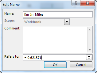
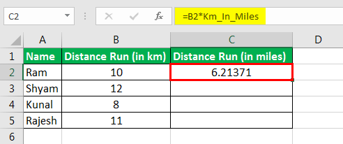
In the “Name Box,” write “Km_In_Miles,” and in the “Refers to” box, specify the value as 0.621371.

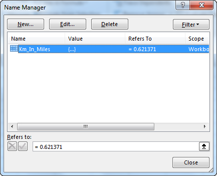
After this, we can see the name “Km_In_Miles” created when we click on the “Excel Name Manager.”

Whenever we want to use a name in a formula, type, and we can see it in the list of suggestions to select.

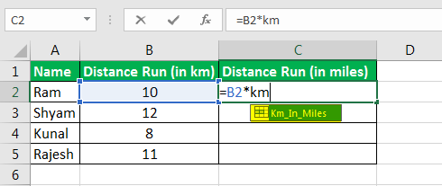
So the answer will be:

Then drag the plus sign to get the answer for all.

Example #3 – Defining Name for a formula

Similar to the above, we can give a name to an Excel formula.

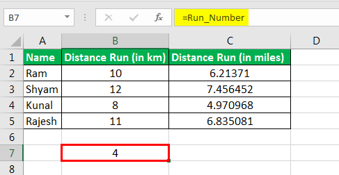
Suppose column A contains the names of people who participated in the run. We want to know the number of people who participated. So, let us create a named formula for it.

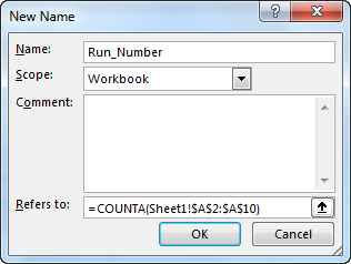
Create a named range “Run_Number” following the above-given steps. So, in the “New Name” window, write the following attributes and click “OK.”

Then use this named range as follows. It may give us the correct number of participants.

Note: If the cells referred to are in the current sheet, then we do not need to mention the sheet number in the Excel formula. However, add the sheet’s name followed by the exclamation point before the cell/range reference if we refer to cells on a different worksheet.

Rules for Name Manager in Excel

Under 255 characters
It cannot contain spaces, and most punctuation characters.
It must begin with a letter, underscore (“_”), or backslash (“”).
It cannot have names like cell references. For example, B1 is not a valid name.
The names are case-insensitive
We can use a single letter name to name a range. However, they can’t be “c,” “C,” “r,” or “R.”

Scope Precedence

The worksheet level takes precedence over the workbook level.

The scope of Excel’s name can be either at the worksheet level or the workbook level.

Worksheet level name is recognized only within that worksheet. Therefore, to use it in another worksheet, we need to prefix the worksheet name followed by an exclamation to the named range.

The workbook level name is recognized in any of the worksheets inside a workbook. Therefore, to use another workbook’s name range in another workbook, we need to prefix the workbook name, followed by an exclamation mark to the named range.

Example #4 – Filters in Excel Name Manager

Excel Name Manager also has the filter functionality to filter out the relevantly named ranges. Please see the screenshot below.

Here, we can see the relevant criteria for filtering the relevantly named ranges. Then, we must select the one we want to restrict to and do whatever we want.

Things to Remember

We must first open Excel Manager: “Ctrl + F3.”
To get a list of all Excel named ranges, we must use F3.
The named ranges are case-insensitive.