Concatenate Strings In Excel

Last Updated :

Blog Author :

Edited by :

Reviewed by :

Table Of Contents

What Is Excel String Concatenation?

The Concatenate Strings in Excel helps users join cell values with text or strings to form combined information of related data or a meaningful sentence.

Excel String Concatenation merges the selected cells, irrespective of the cell values such as text, string, characters, symbols, etc.

For example, to concatenate the two strings “Anand” and “Singh”,

We use the formula =“Anand”&“Singh” using the ampersand (&) symbol, or
We use the formula =Concatenate(“Anand”, “Singh”)

We will get the same output as “Anand Singh”.

Playvolume00:00/00:45TruvidfullScreen

Concatenate Strings in Excel helps users to combine cell values with strings, text, characters, or any other related information to form complete or meaningful sentences.
We can combine cells with any values using the Ampersand (&) and the CONCATENATE function. However, the output is always a Text String irrespective of the cell values such as numbers, dates, etc.
The CONCAT function works with Excel 2016 or above version, and the Concatenate Function is available as the Compatibility function. Therefore, if we are working on the earlier versions of Excel, we must use the Concatenate Function.

How To Do Excel String Concatenation?

We can Concatenate Strings in Excel using 2 methods, namely:

#1 - Using the Ampersand (&) operator -

We select the cell values, and in-between the values, keep adding the & symbol. Therefore, the formula will look as =“cell_value1”&“cell_value2”&“cell_value2”… and so on.

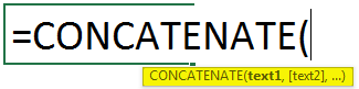
#2 - Using the Concatenate Function -

We can use the inbuilt Concatenate Function in Excel.

The syntax of the Concatenate Function is,

The arguments of the Concatenate Function are,

text1 is the first string to concatenate in Excel.
text2 is the second string to concatenate with text1.

Like this, we can combine 255 values.

Examples

We will consider some examples to Concatenate Strings in Excel.

Example #1 – Basic Example of Concatenating Values into One

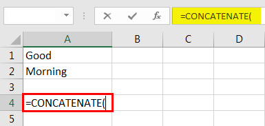
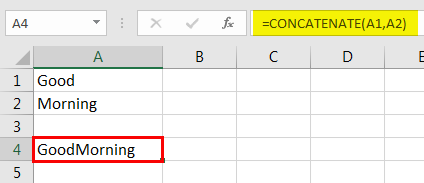
For example, in cell A1 we have “Good”, and in cell A2, we have “Morning”.

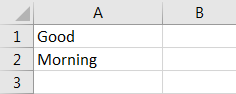
In cell A4, we will combine these two and create a sentence as “Good Morning”.

First, we must open the concatenate formula in cell A4.
Then, select cell A1 as the first argument (Text1).
Next, select cell A2 as the second argument (Text2).
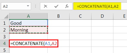
We have only two values to combine. So, close the bracket, and press the “Enter” key. We get the output as “GoodMorning” without a space, as shown below.

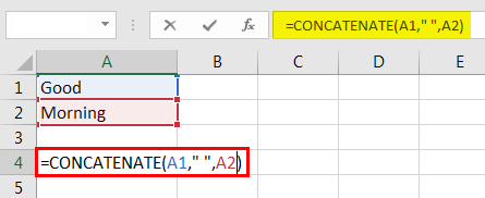
We have selected two values above, so the Concatenate Function combines these two values. So, while applying the formula after selecting Text1, we must insert a space character as the second value to be concatenated before choosing Text2.
After selecting Text1 in the Text2 argument, we must supply the space character in double-quotes as “ ”.
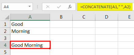
Once the space character is inserted, we will get the following result.

Example #2 – Use the Ampersand (&) Symbol as the Alternative

We can use an ampersand symbol to concatenate values.

For the same example considered above of combining “Good Morning”, we can use the formula below.

After each value, we must put the ampersand (&) symbol. It is the most commonly used method to Concatenate Values in Excel. However, the CONCATENATE formula is not popular among Excel users thanks to the ampersand symbol.

Example #3 – CONCATENATE Cell Values with Manual Values

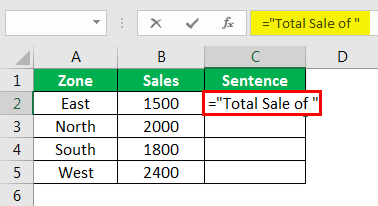
We can enter our values with cell values, like inserting space characters. For example, look at the below data set.

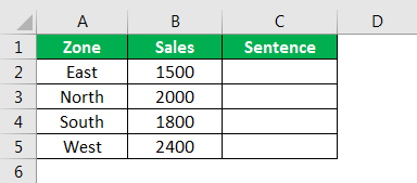
We have a zone-wise sales value here. In the sentence column, we must create a sentence like this –

“Total Sale of East Zone is 1500″

In the above sentence, we have only two values available with cells, i.e., bold values—the remaining values we must add as our own.

We must insert an equal sign in cell C2 to start the concatenation. As part of our sentence, our first value to be concatenated is “Total Sale of “(including space after).

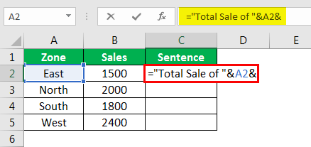
The next value is our cell reference.

The third sentence to be concatenated is "Zone is ".

And the final value is cell reference.

Next, press the “Enter” key to get the output.

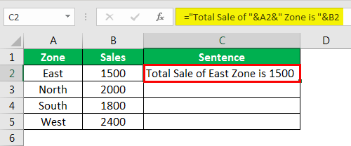
We will drag the formula to get the concatenate values in other cells.

Example #4 - CONCATENATE Date Values

Now, let us consider another example of concatenating dateTEXT function in excel. So, we must select the TEXT function while selecting the “DATE” cell.

Concatenate Strings in Excel example 4.6

Now, we must mention the format as “DD-MMM-YYYY”.

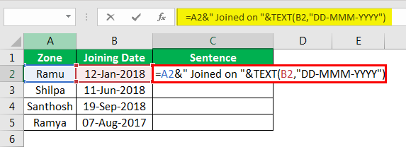
Concatenate Strings in Excel example 4.7

Then, press the “Enter” key to get the answer.

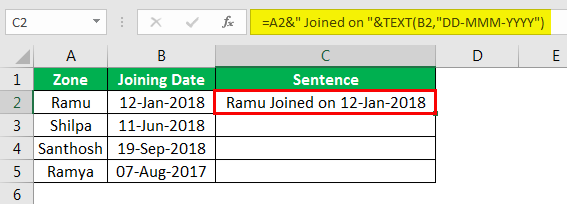
Concatenate Strings in Excel example 4.8

We must apply the TEXT function to the given format as a date because Excel stores date and time as serial numbers. So, whenever we combine, we must provide formatting to them.

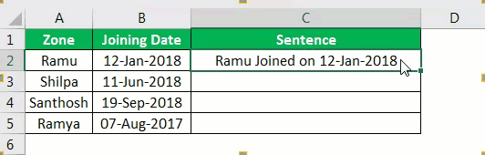
Now, drag the formula to get the concatenate values in other cells.

The output is shown below.

Concatenate Strings in Excel Example 4.9

Important Things To Note

Concatenate Function requires a minimum of one argument to execute. However, it makes sense to have two or more cell values to successfully join the data.
We will get the #Value! error if any one of the selected cell values is invalid.

Frequently Asked Questions

1. Where is the Concatenate Function found in Excel?

First, choose an empty cell - select the “Formulas” tab - go to the “Function Library” group - click the “More Functions” option drop-down - click the “Compatibility” option right-arrow - select the “Concatenate” function, as shown below.

Concatenate String in Excel FAQ 1

2. When we Concatenate Strings in Excel, what cell value limit can we enter?

In the Concatenate Function, we can use a maximum of 8192 characters, i.e., we can concatenate up to 255 Strings. Also, there is no limitation of the 255 strings while using the “&” operator.

3. Why are the Concatenate Strings in Excel not working?

The Concatenate Strings in Excel may not work for the following reasons,
• We would have selected a cell range instead of individually selecting cell values when using the CONCATENATE Function. We must remember that in Concatenate, each cell must be selected independently, as it doesn’t accept arrays or cell ranges.
• One of the arguments might be a numeric value, and the output will have the pre-set Excel serial number remembered by Excel instead of the date. We can change the formatting to get the right result using the Text function, as seen in Example 4.

Download Template

This article must help understand Concatenate Strings in Excel with its formulas and examples. You can download the template here to use it instantly.