RIGHT Function in Excel
The RIGHT function is a text string function that gives the number of characters from the right side of the string. It helps extract characters beginning from the rightmost side to the left. The result depends on the number of characters specified in the formula.
For example, “=RIGHT(“APPLES”,2)” gives “ES” as the result.
Similar to the RIGHT function, the LEFT function in excel returns the characters from the left side of the string.
Syntax
The syntax of the RIGHT function is stated as follows:
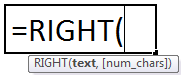
The RIGHT function accepts the following two arguments:
Key Takeaways
- Text: The text string that contains the characters to be extracted.
- Num_chars: The number of characters to be extracted from the string starting from the rightmost side.
The “text” is a mandatory argument and “num_chars” is an optional argument.
The Characteristics of “Num_Chars”
The features of “num_chars” are listed as follows:
- The default value of “num_chars” is set at 1. This means that if the value of “num_chars” is omitted, the RIGHT function returns the last letter of the string.
- If “num_chars” is greater than the length of the text, the RIGHT function returns the complete text.
- If “num_chars” is less than zero, the RIGHT function returns the “#VALUE! error.”
Note: The RIGHT function should not be used with numbers. Though it performs the same operation on digits as it does with text, it returns wrong values with numbers formatted as text.
How To Use RIGHT Function in Excel?
The RIGHT function is mostly used in combination with other Excel functions like FIND, SEARCH, LEN, LEFT, etc.
The uses of the RIGHT function are listed as follows:
- It removes the trailing slash in URLs.
- It extracts the domain name from the email address.
- It helps format text.
- It extracts text occurring after a specific character.
Example #1
A text string is given in cell A3, as shown in the succeeding image. We want to extract the last word having six letters.
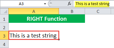
Let us apply the RIGHT formula to extract “string” in A3.
We use “=RIGHT(A3,6).”

The RIGHT formula returns “string.”
Example #2
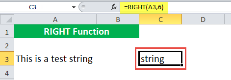
The following image shows a list of IDs like “ID2101,” “ID2102,” “ID2103,” etc., in column A.
Here, the last four digits of the ID are unique and the text “ID” is redundant. So, we want to remove “ID” from the list of identifiers.

We apply the formula “=RIGHT(A3,4).”

The RIGHT function returns 2101 in cell B3. In the same way, we extract the last four digits of all the IDs.
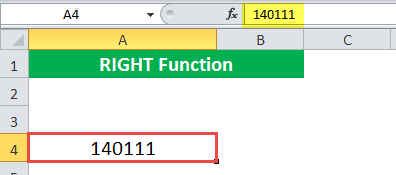
Example #3
We have a 6-digit number (140111) and want to extract the last 3 digits from this number.
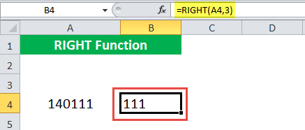
We apply the formula “=RIGHT(A4,3)” to extract the last three digits.
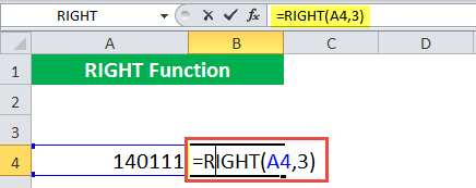
The RIGHT function returns 111.
Example #4
We have the date “12/07/2018” in cell A5. We want to extract the last few digits.
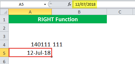
To extract the last three digits, we apply the formula “=RIGHT(A5, 3).”
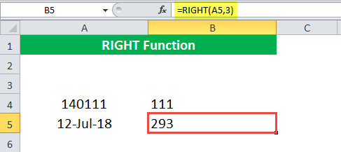
The function returns 293 instead of 018. This is because it considers the original value of the date before returning the output. So, the RIGHT function does not give the correct answer in this case.
Example #5
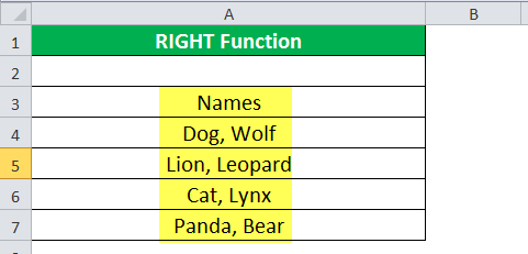
We have the names of two animals in column A. The names are separated by a comma and space, as shown in the following image. We want to extract the last name.
We apply the following RIGHT formula.
“=RIGHT(A4,LEN(A4)-FIND(“ ”,A4))”
The “FIND(“ ”,A4)” finds the location of the space. It returns 5. Alternatively, we can use “,” for a stricter search.
The “LEN(A4)” calculates the length of the string “Dog, Wolf.” It returns 9.
The “LEN(A4)-FIND(“ ”,A4)” returns the position of the space from the right. It returns 4.
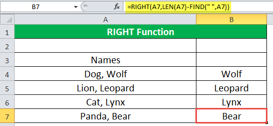
The formula “RIGHT(A4,LEN(A4)-FIND(“ ”,A4))” returns four letters from the right of the text string in A4.
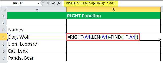
The output of the RIGHT formula is “Wolf.” Similarly, we find the output for the remaining cells as well.
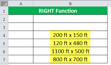
Example #6
We have two-dimensional data, the length multiplied by the width, as shown in the following image. We want to extract the width from the given dimensions.
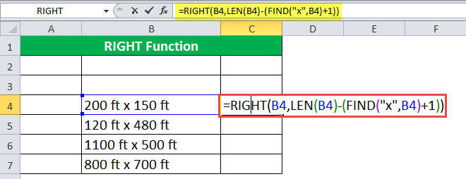
For the first dimension, we apply the following RIGHT formula.
“=RIGHT(B4,LEN(B4)-(FIND(“x”,B4)+1))”
The “FIND(“x”,B4)” gives the position of “x” in the cell. It returns 8.
The formula “FIND(“x”,B4)+1” returns 9. Since “x” is followed by a space, we add one to omit the space.
The “LEN(B4)” returns the length of the string.
The “LEN(B4)-(FIND(“x”,B4)+1)” returns the number of characters occurring after “x”+1.
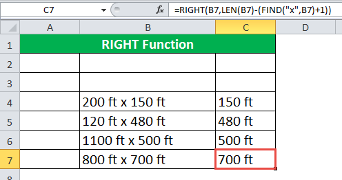
The formula “RIGHT(B4,LEN(B4)-(FIND(“x”,B4)+1))” returns all the characters occurring in one place after “x.”
The RIGHT formula returns “150 ft” for the first dimension. Drag the fill handle to get the results for the remaining cells.
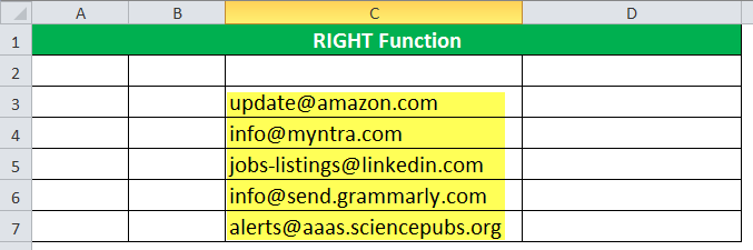
Example #7
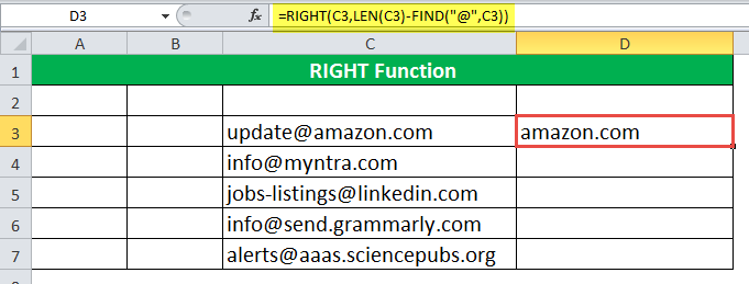
We have a list of email addresses. We want to extract the domain name from these email IDs.
We apply the following RIGHT formula to extract the domain name from the first email address.
“=RIGHT(C3,LEN(C3)-FIND(“@”,C3))”
The “FIND(“@”,C3)” finds the location of “@” in the string. For cell C3, it returns 7.
The “LEN(C3)” gives the length of the string C3. It returns 17.
The “LEN(C3)-FIND(“@”,C3)” gives the number of characters occurring to the right of “@.” It returns 10.
The “RIGHT(C3,LEN(C3)-FIND(“@”,C3))” gives the last 10 characters of cell C3.

The RIGHT formula returns “amazon.com” in cell D3.
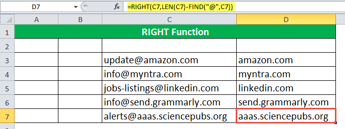
Similarly, we apply formulas to the remaining cells as well.
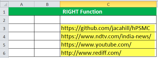
Example #8
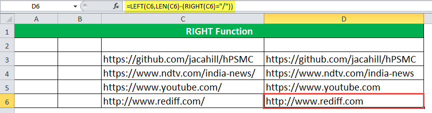
We have some URLs shown in the following image. We want to remove the last backslash from these URLs.
We apply the following formula.
“=LEFT(C3,LEN(C3)-(RIGHT(C3)=”/”))”
By default, the RIGHT function returns one value on the rightmost side, i.e., the last value.
If the last character is a forward slash (/), “(RIGHT(C3)=”/”)” returns “true,” else it returns “false.” These “true” and “false” change to one and zero, respectively.
If the last character is a forward slash (/), one is subtracted from the length of the string. This means that if the last character is “/”, the “LEN(C3)-(RIGHT(C3)=”/”))” omits it.
The “=LEFT(C3,LEN(C3)-(RIGHT(C3)=”/”))” returns the first “n” number of characters. If the last character is a forward slash (/), it is omitted; else, the complete string is returned.
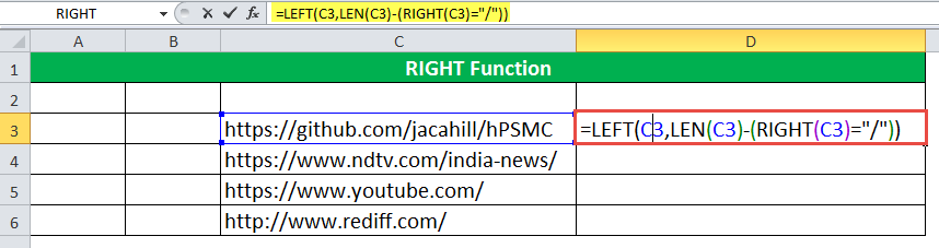
The formula returns the complete string in cell D3.

Similarly, we apply formulas to the remaining cells as well.
Frequently Asked Questions (FAQs)
#1 – What are the LEFT, RIGHT, and MID functions in Excel?
The LEFT and RIGHT functions extract characters or substrings from the left and the right side of the source string, respectively. The MID function extracts characters from the middle of the string.
The syntax of the three functions is stated as follows:
“=LEFT(text, )”
“=RIGHT(text, )”
“=MID(text, start_num, num_chars)”
The arguments are explained as follows:
– Text: The actual text string that contains the characters to be extracted. This is usually in the form of a cell reference.
– Num_chars: The number of characters to be extracted from the string.
– Start_num: The position within the source data string from where the extraction should
begin.
#2 – How to remove characters by using the RIGHT function in Excel?
The number of characters to be removed is subtracted from the total length of the string. For this, the following formula is used:
“=RIGHT(string,LEN(string)-number_of_chars_to_remove)”
The “string” is the entire source string. The “number_of_chars_to_remove” contains the number of characters to be removed from the source string.
#3 – How to use the RIGHT function for numbers in Excel?
The RIGHT function always returns a text string even if the source string is in the form of numbers. To get the output as a number from a string of numbers, the RIGHT function is nested in the VALUE function.
The formula is stated as follows:
“=VALUE(RIGHT(string, num_chars))”
The “string” is the source string containing numbers. The “num_chars” is the number of digits to be extracted from the string.
Note: In Excel, the numbers string is right-aligned while the text string is left-aligned.
- The RIGHT function gives a specified number of characters from the right side of a text
string. - The RIGHT function extracts characters beginning from the rightmost side to the left.
- The RIGHT function accepts two arguments–“text” and “num_chars.”
- The default value of “num_chars” is set at 1.
- If “num_chars” is greater than the length of the text, the RIGHT function returns the complete text.
- If “num_chars” is less than zero, the RIGHT function returns the “#VALUE! error.”
- The RIGHT function should not be used with numbers because it returns wrong values
with numbers formatted as text.
Recommended Articles
This has been a guide to RIGHT Function in Excel. Here we discuss the RIGHT Formula in Excel and how to use the RIGHT Excel function along with Excel examples and downloadable Excel templates. You may also look at these useful functions in Excel –