Opposite Of Concatenate In Excel

In our earlier article, “Concatenate Strings in Excel,” we have seen how to combine values of more than one cell into one with various practical examples. However, have you ever thought about what would be the complete opposite of concatenating in Excel?

Yes, we can do the opposite of concatenating in Excel. We have several methods to do this job. First, this article will show how to split one cell's data into multiple cells.

For example, consider the below example showing a name in column A. Let us learn how to split the name into other cells.

The steps are:

Step 1: First, select the cell which we want to split.

Step 2: Next, go to Data - Text to Columns in Excel.

Step 3: Now, the window, Convert Text to Columns Wizard – Step 1 of 3 appears.

Step 4: Next, select Delimited in Convert Text to Columns Wizard – Step 2 of 3.

Step 5: Then, select Space in Convert Text to Columns Wizard – Step 3 of 3 since the first and last names are separated by a space.

Step 6: Now, click on Finish.

Likewise, we can split data into other cells.

In this article will show how to split one cell’s data into multiple cells.

• Opposite of concatenate in Excel refers to the method to split data from one cell into other cells.
• To split data from one cell to others, we can use Excel TEXT functions, such as RIGHT, LEFT functions.
• Alternatively, we can use Text to Columns in Excel method to split data into other cells.
• While using text to columns in Excel method, we can split content on the basis of tab, semicolon, comma, and space.
• If there is any other symbol used to divide text, we can use the Other: option to specify.

Below are the examples of excel opposite to concatenate.

Method #1 – Split Values By Using Text Functions

Excel TEXT functions are popular ways to split one cell value into multiple cells. Excel’s LEFT function, RIGHT function, and MID function in excel are popular text functions.

We are using the below data for this example.

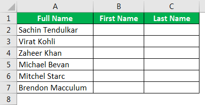
We have the full name of cricketers here. However, we need first to extract the first name here. We can do this by applying the LEFT function in Excel and FIND excel function because once the value to be split is selected; we must specify the number of characters we need to extract from the left side of the selected data.

Like this, we can do the opposite of concatenating in Excel. We can also do the opposite of concatenating with another method, “Text to Column.”

Method #2 – Opposite Of Concatenate Through Text To Column

It is the best example of a simple procedure. In addition, this method does not involve any complex formulas. We will see this in the below example.

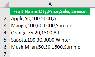
The above data should be in the below format.

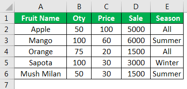
It looks like one hell of a task.

But actual work is easier than we assume. By using the one common thing, which is combining this data, we can split accordingly. In this case, the common thing combining different columns into one is a comma (,).

To begin with, we must select the data.

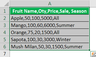
Then, go to Data > Text to Columns in excel. Else, we can press the excel shortcut key ALT + A + E.

Next, we can see the below window when we click on “Text to Columns.”

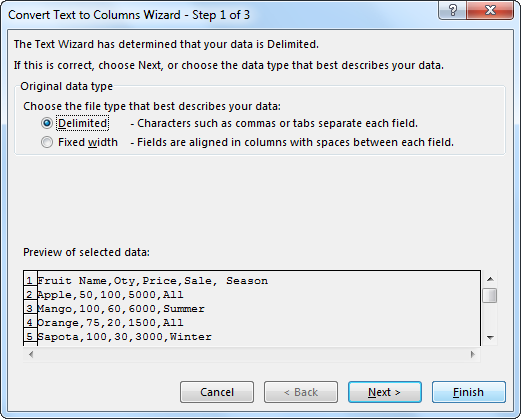
Now, select “Delimited,” and then, click on “Next.”

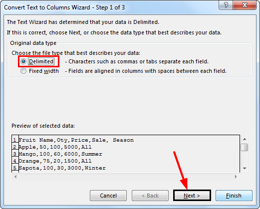
Now, in the second window, we need to select the Delimiter, the common thing, combining all the columns into one. Therefore, in this case, “Comma,” so select comma.

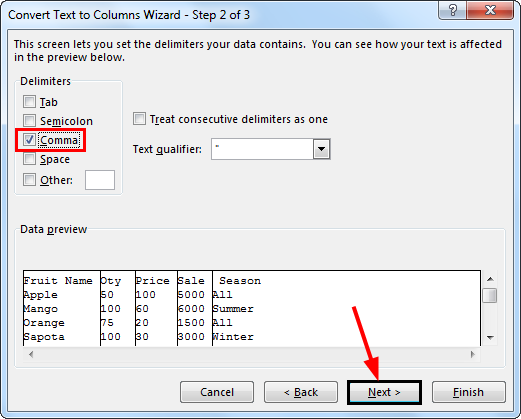
Now, click on “Next” and then, click on “Finish” in the next window. We will get the opposite of the concatenate.

Likewise, we can use functions and “Text to Columns” in Excel to do the opposite of concatenating.

Example #1

For example, consider the below example showing an employee’s name, age and country in column A. Let us learn how to split the name into other cells.

The steps are:

Step 1: First, select the cell which we want to split.

Step 2: Next, go to Data - Text to Columns in Excel.

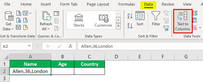
Step 3: Now, the window, Convert Text to Columns Wizard – Step 1 of 3 appears.

Step 4: Next, select Delimited in Convert Text to Columns Wizard – Step 2 of 3.

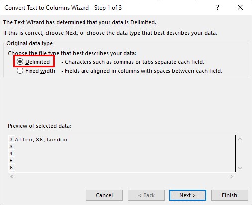
Step 5: Then, select Space in Convert Text to Columns Wizard – Step 3 of 3 since the first and last names are separated by a comma.

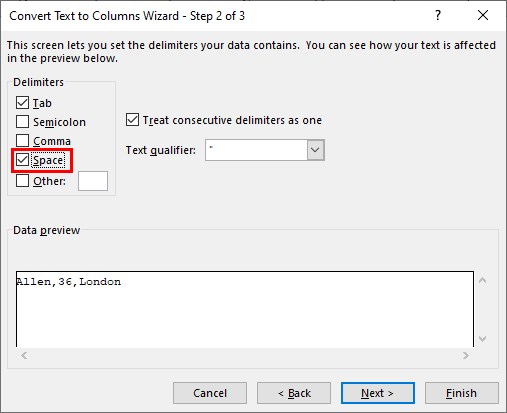
Step 6: Now, click on Finish.

Likewise, we can split data into other cells.

Example #2

Consider the below table showing list of Phd scholars in an university. Now, let us learn how to split the text into First Name and Last Name using TEXT functions in Excel.

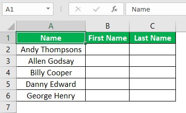
The steps are:

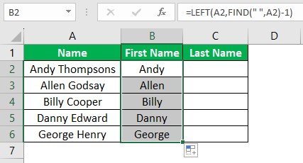
First, we need to extract the first name in cell B2. We can do this by applying the LEFT function in Excel and FIND excel function.

So, insert the formula, =LEFT(A2,FIND(“ "A2)-1)

 Then, press Enter key.

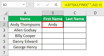
Finally, we can see the result in cell B2.

Now, using AutoFill option, we can obtain the results in other cells.

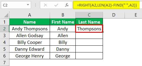
Next, let us extract the last name in cell C2.

Then, insert the formula, =RIGHT(A2,LEN(A2)-FIND(" ",A2)) in cell C2.

Next, press Enter key. We can see the result in cell C2.

Next, using AutoFill option, we can obtain the results in other cells.

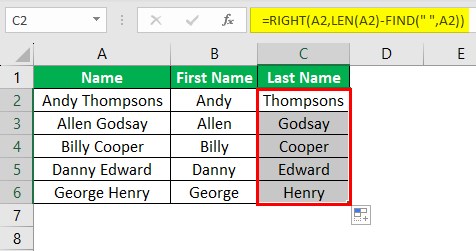
Like this, we can do the opposite of concatenating in Excel.

Example #3

For example, consider the below example showing product, price and stock availability in column A. Let us learn how to split the text into other cells.

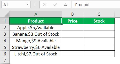
The steps are:

Step 1: First, select the cell which we want to split.

Step 2: Next, go to Data - Text to Columns in Excel.

Step 3: Now, the window, Convert Text to Columns Wizard – Step 1 of 3 appears.

Step 4: Next, select Delimited in Convert Text to Columns Wizard – Step 2 of 3.

Step 5: Then, select Space in Convert Text to Columns Wizard – Step 3 of 3 since the first and last names are separated by a comma.

Step 6: Now, click on Finish.

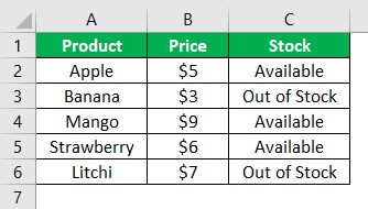
Likewise, we can split data into other cells.

• To split text into columns, we need to select Data tab.
• Then, click on Text to Columns in Excel option.
• Select Delimited and click on the desired delimiters.

This article is a guide to the Opposite of Concatenate in Excel. We discuss the top 2 methods to opposite concatenate 1) Text functions and 2) Text to Columns method in Excel with examples and a downloadable Excel template. You may learn more about Excel from the following articles: -

• Excel AVERAGEIFS Function
• Count Characters in Excel Cell
• Substitute Formula In Excel
• Combine Cells in Excel

This article must be helpful to understand the Excel Column Auto Width, with its formula and examples. You can download the template here to use it instantly.