Table Of Contents
Excel REPT Function
The REPT function is also known as the repeat function in Excel. As the name suggests, this function repeats the provided data according to the given number of times. So, this function takes two arguments: the first is the text that needs to be repeated, and the second is the number of times we want the text to be repeated.
For example,=REPT("p",3) returns "ppp."
Syntax
Below is the REPT formula in Excel.

Arguments
- text = It is a required parameter. It is the text to be repeated.
- number_of_times = It is also a required parameter. It is the number of times the text in parameter-1 is to be repeated. It must be a positive number.
Examples to use REPT Function in Excel
The REPT function is a Worksheet (WS) function. Therefore, the REPT function can be inserted as a part of the formula in a worksheet cell as a WS function. Refer to a couple of examples given below to know more.
Example #1 - Repeat a set of characters

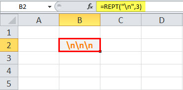
In the above example, REPT(“\n,” 3) “n” is said to be repeated 3 times. As a result, cell B2 contains “nnn.”
Example #2 - Repeat a character

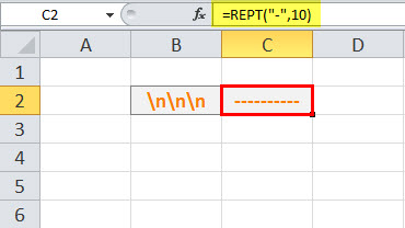
In the above example, REPT (“-,” 10) “-” is said to be repeated 10 times. As a result, cell C1 contains “———-.”
Example #3 - Equalize the length of the numbers

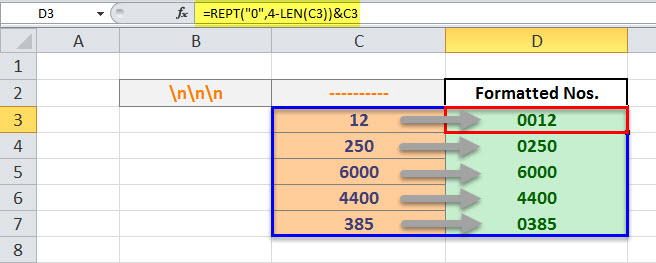
In the above example, column C contains a series of numbers from C3 to C7.
The number of digits each cell contains is different. So, the use case is to make all the numbers of the same length by adding zeros (0) so that the value of the number does not change, but all the numbers become of the same length.
Here, the length defined is 4. That is, all the numbers should be of length 4. The formatted numbers are in column D, starting from D3 to D7. So, the formatted number of C3 is present in D3, C4 in D4, C5 in D5, C6 in D6, C7 in D7, and so on. Each cell from D3 to D7 has a REPT function applied to it.
Here, the REPT function is used to add leading or trailing zeros. First, let us analyze the REPT function written in the formula bar.
=REPT(“0”,4-LEN(C3))&C3
As shown in the above REPT formula in Excel, “0” represents a digit/text to be repeated. The second parameter is the frequency with which zero is to be repeated. Here, the length of the number in the C3 cell is deducted from number 4, which will give us the number of zeros to be repeated to format the number in 4-digit format.
E. g: If the length of the number present in C3 is 2, then 4-2=2, which is evaluated to – REPT (“0”,2), meaning repeat 0 twice. Further, the resultant number ends with the original value, which here is 12, and the result is 0012.
Example #4 - Create in-cell charts

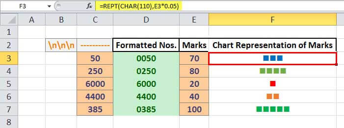
In the above example, column E contains a series of marks obtained out of 100 from E3 to E7. Therefore, it will represent the marks obtained in a graphical format without using the default charts widget in Excel. We can accomplish it by using the REPT function, as explained below.
Here, the REPT formula is =REPT(CHAR(110), E3*0.05).
All characters have an ASCII code, which is understood by the computer. For example, small case ‘n’ has code 110. So, =CHAR (110) in Excel returns ‘n.’ When "Wingdings" font is applied on the same, it becomes a block displayed as – n.
Now, we have got the character to be repeated. Now, we must figure out how many times it is to be repeated. So, the REPT function is applied to calculate the number of blocks: – E3*0.05, meaning one block would represent 1/5th of the value. So, the number of blocks for marks 70 is shown as 3 repeated blocks in the result cell F3.
A similar formula is repeated on the remaining values, from E4 to E7, resulting in 4, 1, 2, and 5 blocks for marks 80, 20, 40, and 100 shown in the result cells F4, F5, F6, F7, respectively.
Things to Remember
- The second parameter of the REPT function must be a positive number.
- If it is 0 (zero), the REPT function returns “” i.e., an empty text.
- If it is not an integer, it is truncated.
- The result of the REPT function cannot be longer than 32,767 characters. Else, the REPT formula returns #VALUE! Error indicating an error with the value.

