Hyperlink Excel Function

Last Updated :

21 Aug, 2024

Blog Author :

Edited by :

Reviewed by :

Table Of Contents

What is HYPERLINK Function in Excel?

The HYPERLINK function of Excel helps create a link (or hyperlink), which when clicked, takes the user to the intended location. Every link is given a desired on-screen name. Once a hyperlink is created, this name is underlined and displayed in blue. Apart from text, a picture can also be turned into a clickable hyperlink.

For example, the formula =HYPERLINK("http://www.wallstreetmojo.com/","WSM") creates a hyperlink named “WSM.” When clicked, this hyperlink opens the website “www.wallstreetmojo.com.”

The purpose of creating a hyperlink in Excel is to provide the end-user with an additional source of information. This source is usually related to the current data of the worksheet. The HYPERLINK function is categorized under the Lookup & Reference functions of Excel.

Table of contents

What is HYPERLINK Function in Excel?

Formula of the HYPERLINK Function of Excel

The formula of the HYPERLINK function of Excel is shown in the following image.

Hyperlink Function formula

The HYPERLINK function of Excel accepts the following arguments:

Link_location: This is the path to the intended location. It can be supplied as a text string enclosed within double quotation marks or a reference to a cell that contains this text string. The intended location can be a cell, named range (in any workbook), bookmark or file in Word, web page on the intranet or Internet, file on Excel or PowerPoint, etc.
Friendly_name: This is the on-screen name of the hyperlink. It is also called the jump text, link text or anchor text. It can be supplied as a text string enclosed within double quotation marks, numeric value or reference to a cell containing the on-screen name. The blue color of the jump text indicates that it is clickable.

The argument “link_location” is required while “friendly_name” is optional. If the latter is omitted, the former is considered as the jump text.

The HYPERLINK formula in excel can return errors in the following situations:

If the path specified as the “link_location” does not exist, an error is displayed on clicking the hyperlink.
If there is an issue with the “friendly_name,” the cell shows an error in place of the jump text.

Hyperlink-Function-in-Excel

Hyperlink Excel Function Video Explanation

Examples

Let us consider a few examples to understand the working of the HYPERLINK function in Excel.

Example #1–Send an Email Using a Hyperlink

To send an email using a hyperlink, follow the listed steps:

Open the HYPERLINK function by typing =HYPERLINK in Excel.
Prefix “mailto:” (within double quotation marks) to an email address. Use the ampersand operator to join this prefix and the cell containing the email address. This serves as the “link_location” argument.
Close the parentheses and press the “Enter” key.

The HYPERLINK formula is displayed in cell C2 of the following image.

Hyperlink EXAMPLE 1-2

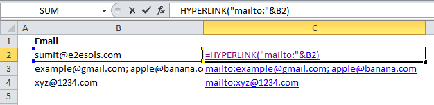
Result of the HYPERLINK formula: The prefix along with the entire address (mailto:sumit@e2esols.com) will be displayed as a hyperlink. Since the “friendly_name” argument has been omitted in the HYPERLINK formula, the “link_location” is used as the jump text.

Clicking the created hyperlink will open the “compose” page of the default email account. The given email address will be automatically entered in the “To” field. This field contains the email address of one or more recipients.

Likewise, the HYPERLINK formula has been applied to cells C3 and C4. The outputs of the HYPERLINK formulas are displayed in these cells. Notice that the “friendly_name” has been omitted for the hyperlinks of these cells as well.

Note: “Mailto” links are used in HTML to send emails from the default mail client of the user. The address mentioned in the “mailto” link is considered to belong to the intended recipient.

Example #2–Switch Between the Worksheets Using a Hyperlink

To switch to a different worksheet within the same workbook via a hyperlink, follow the listed steps:

Open the HYPERLINK function by typing =HYPERLINK in Excel.
Prefix the hash (#), followed by the name of the worksheet, the exclamation mark (!), and the cell reference of the intended location. This serves as the “link_location” argument.
Enter the jump text enclosed within double quotation marks.
Close the parentheses and press the “Enter” key.

The HYPERLINK formula is displayed in cell C5 of the following image.

Hyperlink EXAMPLE 1-3

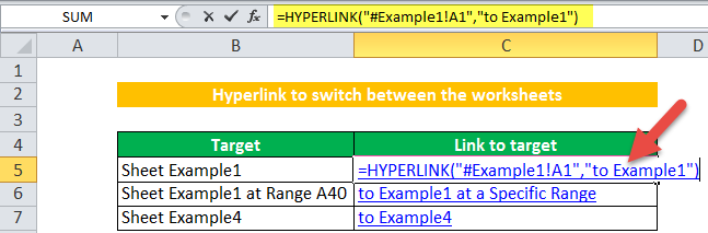
Result of the HYPERLINK formula: A hyperlink with jump text “to Example1” will be created. Clicking this hyperlink will take the user to cell A1 of the worksheet “Example1.” In this way, one can move within a workbook through hyperlinks.

Likewise, the hyperlinks of cells C6 and C7 will take the user to the intended locations given in cells B6 and B7 respectively.

Therefore, hyperlinks can be used to link the table of contents of a workbook to the different areas of worksheets.

Alternate Method to Switch Between the Worksheets

This section lists the alternative steps to the preceding method. The steps to switch to a different worksheet (within the same workbook) by using a hyperlink are listed as follows:

Type the jump text in a cell. Next, select this cell.
Click the “hyperlink” option from the “links” group of the Insert tab.
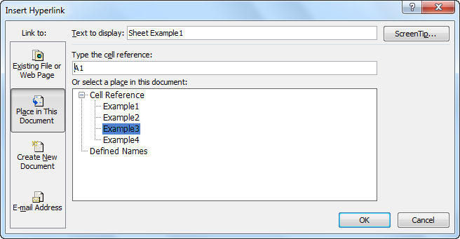
The “insert hyperlink” dialog box opens. Under “link to” displayed on the left side, select “place in this document.”
In “text to display,” Excel automatically displays the selected jump text. In “type the cell reference,” enter the cell reference of the intended location.
Under “or select a place in this document,” choose the worksheet where the user would be taken.
Click “Ok.”

The “insert hyperlink” dialog box is shown in the following image. In this case, clicking the jump text “Sheet Example1,” will take the user to cell A1 of worksheet “Example3.”

Hyperlink EXAMPLE 1-4

Example #3–Open a File Using a Hyperlink

To open a file through a hyperlink, follow the listed steps:

Open the HYPERLINK function by typing =HYPERLINK in Excel.
Enter the reference to a cell containing the full path of the file. The path should include the location, name, and extension (like .docx, .xlsx, .pptx, and so on) of the file. This serves as the “link_location” argument.
Enter the jump text enclosed within double quotation marks.
Close the parentheses and press the “Enter” key.

The HYPERLINK formula is displayed in cell C3 of the following image.

Hyperlink EXAMPLE 1-5

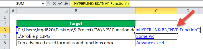
Result of the HYPERLINK formula: A hyperlink with jump text “NVP Function” is created. Clicking this hyperlink opens the file titled “NPV function.” This file is currently stored on the desktop of the user.

Likewise, the hyperlink of cell C4 opens an image having the “.jpg” extension. The hyperlink of cell C5 opens a Word document titled “top advanced excel formulas and functions.”

While this discussion provides a solid overview, engaging with more in-depth material can significantly enhance this comprehension. Many find that this Excel Hacks and Tips Course complement this knowledge beautifully.

How to Make a Picture or Cell of Excel a Clickable Hyperlink?

Let us learn how to make a picture or cell of Excel clickable. Note that the procedure of creating hyperlinks in both cases is the same.

The steps to make a picture or cell of Excel clickable are listed as follows:

Select the picture or the cell containing the text which needs to be made clickable. Right-click the selection and choose “hyperlink” from the context menu.

The selection and “hyperlink” option are shown in the following image. Note that the green box shown on the left side is currently not clickable. This box is just an ordinary picture of Excel, which has been inserted from the “picture” option (“illustrations” group) of the Insert tab.

Note: Alternatively, after selecting the cell or picture, one can click “hyperlink” from the “links” group of the Insert tab.
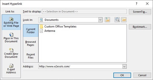
The “insert hyperlink” dialog box opens. Enter the path or the “link_location” in the address box and click “Ok.” The options “existing file or web page” (under “link to”) and “current folder” (under “look in”) automatically appear to be selected. Let them remain the way they are.

We have entered the path as “http://www.e2esols.com/,” as shown in the following image. As one begins to type “www” in the address box, Excel automatically inserts “http,” colon (:), and forward slashes (/) at the right places. So, when the user clicks on the picture (shown in step 1), he/she will be taken to this website.

In this way, a picture or cell of Excel can be turned into a clickable hyperlink. Note that the position or the appearance of the picture is not impacted. It has only been made clickable.

Note: The web address or URL (uniform resource locator) entered in this example does not exist. This URL has been used for example purposes only.

The Key Points Governing Hyperlink Formula in Excel

The important points related to creating hyperlinks in Excel are stated as follows:

The “insert hyperlink” dialog box (opens by clicking “hyperlink” on the Insert tab) shows a “screen tip” option on the top-right side. When clicked, it allows the user to enter information related to the hyperlink. This information is displayed when the cursor rests on the hyperlink and changes to a hand icon.
It is possible to select a cell containing a hyperlink without being taken to the intended location. This can be done by following either of the stated methods:
- Select an adjacent cell and use the arrow keys to select the cell containing the hyperlink.
- Click the required cell (containing the hyperlink) and keep the mouse button pressed until the cursor assumes a “plus” or “cross” sign. Once this sign is displayed, release the mouse button.

Frequently Asked Questions

1. Define the HYPERLINK function of Excel with the help of an example.

The HYPERLINK function helps create hyperlinks in Excel. When such a hyperlink is clicked, it takes the user to a different web page, document, bookmark, workbook, and so on. By creating a hyperlink in a worksheet, the end-user is given access to an additional source of data.

For example, the formula =HYPERLINK(“http://www.123.com/”,123) creates a hyperlink named 123. When this link is clicked, the stated website (www.123.com) opens.

Note: For more details on the usage of the HYPERLINK function, refer to the examples of this article.

2. How to use the HYPERLINK function in Excel?

The HYPERLINK function of Excel can be used by following the listed steps:
a. Open the HYPERLINK formula by typing =HYPERLINK in Excel.
b. Enter the path of the destination. This is the place where the user would be taken on clicking the hyperlink.
c. Enter the name of the hyperlink, which will be displayed to the user. If the name is not entered, the path will be displayed as the name.
d. Close the parentheses and press the “Enter” key.

Note: For more details on the arguments of the HYPERLINK excel formula, refer to its syntax given in this article.

3. Where is the “hyperlink” button and how is it used to add a hyperlink in Excel?

The “hyperlink” button is in the “links” group of the Insert tab. It is used to add a hyperlink to a blank cell, cell containing a string (whether textual or numerical) or cell containing an image.

For inserting a hyperlink using the “hyperlink” button, follow the listed steps:
a. Select the cell or image on which a hyperlink needs to be created.
b. Click the “hyperlink” button from the Insert tab or the “hyperlink” option from the context menu. The context menu appears when the selected cell or image is right-clicked.
c. The “insert hyperlink” dialog box opens. Enter a name for the hyperlink in the “text to display” box.
d. Enter the address in the address box. This address is the URL of a web page.
e. Click “Ok.”

A hyperlink is created using the “hyperlink” button of Excel. In case, an image was selected in pointer “a,” it becomes clickable.

Note: While creating this hyperlink, let the default selections of Excel (“existing file or web page” under “link to” and “current folder” under “look in”) stay in place. The other options under “link to” can also be used depending on the kind of destination.