How to Unhide Columns in Excel?

Last Updated :

Blog Author :

Edited by :

Reviewed by :

Table Of Contents

7 Methods to Unhide Columns in Excel

By hiding the data, the selected columns disappear from the display. However, the labels of the remaining columns stay the same. In addition, a thick bar in the column header area appears to indicate the hidden columns.

It is essential to know the techniques to unhide data. The seven ways to unhide Excel columns are stated as follows:

Home tab of Excel ribbon
Shortcut key
Context menu
Column width
Ctrl+G (go to) command
Ctrl+F (find) command
Double-line icon

7 Methods to Unhide Columns in Excel

In the given techniques, the method names followed by the steps to unhide are listed.

Method #1–Home Tab of Excel Ribbon

Select the columns to the left and right of the hidden column.
In the Home tab, under the “cells” group, click the “format” dropdown.
From the “hide and unhide” option, select “unhide columns.”

Method #2–Shortcut Key

Select the columns to the left and right of the hidden column.
Press the shortcut “Alt H O U L.” Press one key at a time.

Method #3–Context Menu

Select the columns to the left and right of the hidden column.
Right-click on the selected columns and choose “unhide.”

Method #4–Column Width

Select the columns to the left and right of the hidden column.
Right-click on the selected columns and choose “column width.”
Enter any number as the “column width.”

Method #5–Ctrl+G (Go To) Command

In the succeeding image, column B and C are hidden.

In the Home tab, click “find and select” drop-down and choose “go to.” Alternatively, press the shortcut key F5.
Specify any cell reference of the hidden column like B1:C1 in the “go to” dialog box. Click “Ok.”

Choose any preceding technique (methods #1 to #4) to unhide columns B and C.

Method #6–Ctrl+F (Find) Command

In the succeeding image, column B and C are hidden.

Press “Ctrl+F” and the “find and replace” dialog box appears.
Enter the data of one of the hidden cells in the “find what” box.
Click “options>>” and select the check box “match entire cell contents.”
Click “find next” and close the “find and replace” dialog box.
Select any preceding technique (methods #1 to #4) to unhide columns B and C.

Note: This method works in case the cell reference is unknown and the cell data is known.

Method #7–Double-line Icon

Enter a single cell reference of the hidden column in the “name” box. This is the box to the left side of the formula bar.
Press the “Enter” key.
Select the columns to the left and right of the hidden column.
Double-click the double-line icon (having arrows pointing to the left and right) in-between the column labels. Alternatively, follow method#1 to unhide the column.

Unhide the First Column in Excel

It is difficult to select and unhide the first column (column A). To unhide all the hidden columns in one go, follow method #1.

The steps to unhide only the first column are listed as follows:

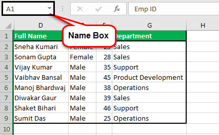
Type A1 in the name box (shown in the succeeding image) and press the “Enter” key. Alternatively, in the Home tab, click “find and select” drop-down and choose “go to.”
In the Home tab, under the “cells” group, click the “format” dropdown.
From the “hide and unhide” option, select “unhide columns.”

Locate and Unhide the Hidden Columns

The steps to locate and unhide the hidden columns are listed as follows:

Select the entire sheet.
In the Home tab, click “find and select” drop-down and choose “go to.” Alternatively, click “go to special.”
Click “special” and select the check box “visible cells only.” Click “Ok.”

The visible part of the table is highlighted (shown in the succeeding image). Moreover, a line between the column labels appears that shows the hidden columns.
Select the highlighted part and follow any preceding technique (methods #1 to #4) to unhide columns B and C.

Create a Custom View

With the “custom view,” a user can save particular display settings. For instance, one user may want to hide columns while the other may wish to view the entire data in one go.

The steps to create a “custom view” are listed as follows:

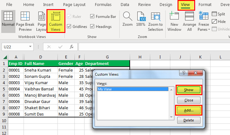
In the View tab, click “custom views,” under the “workbook views” group.
Click “add” and in the “add view” dialog box, enter a name for the view you want to create. The succeeding image shows the “custom view” titled “my view.”
In “include in view,” select the settings of the view and click “Ok.”
The “custom view” titled “my view” is created. Every time you select “my view” and click “show,” the display settings of “my view” become visible.

Hence, with the selection of “my view,” the columns A, D, E, F, and G are displayed, as shown in the succeeding image. The columns B and C are hidden because they were not active when “my view” was created.

Frequently Asked Questions

What does it mean to unhide columns in Excel?

Sometimes it becomes essential to hide particular columns to have a contracted view of the large data set. The option of hiding certain columns is better than deleting them. Before the spreadsheet containing hidden columns goes to the next user, it becomes essential to unhide them for facilitating a complete data view.

The steps to unhide the columns of the entire worksheet in one go are listed as follows:
• Select the entire worksheet by either clicking the triangle to the left of column A or pressing “Ctrl+A.”
• In the Home tab, under the “cells” group, click the “format” dropdown.
• From the “hide and unhide” option, select “unhide columns.”
Hence, all the columns of the worksheet become visible.

How to unhide the first column (column A) in Excel?

The three methods to unhide column A are listed as follows:
1. First method
a. Enter the reference A1 in the name box (to the left of the formula bar). Press the “Enter” key.
b. In the Home tab, under the “cells” group, click the “format” dropdown.
c. From the “hide and unhide” option, select “unhide columns.”
2. Second method
a. Select column B by clicking on its header.
b. Move the cursor to the left of column B till the double-line icon (having arrows pointing to the left and right) in the column header area appears.
c. Drag the double-line icon to the right for expanding column A.
3. Third method
a. In the Home tab, click “find and select” drop-down and choose “go to.” Alternatively, press the shortcut key F5.
b. In the “go to” dialog box, enter A1 in the “reference” box. Click “Ok” and the cell A1 is selected.
c. Follow the steps “b” and “c” of the first method.

How to unhide all Excel rows and columns with a shortcut key?

The steps to unhide all rows and columns with a shortcut key are listed as follows:
• Select the entire worksheet by either clicking the triangle to the left of column A or pressing “Ctrl+A.”
• Press the shortcut “Ctrl+Shift+9” to unhide all rows. Press all keys together.
• Select the entire worksheet again.
• Press the shortcut “Alt H O U L” to unhide all columns. Press one key at a time.