Hide Column in Excel

Last Updated :

Blog Author :

Edited by :

Reviewed by :

Table Of Contents

Hiding Excel Column(s)

Hiding a column in excel implies making it invisible so that it is removed from display. A hidden column is not deleted from the worksheet. This means that it does exist and has been only temporarily held from view. In Excel, one can hide both contiguous and non-contiguous columns. However, to use a hidden column again, it needs to be unhidden at first.

For example, a column containing calculations may be hidden. This helps avoid confusion amongst users of a shared worksheet.

A column is hidden when its data needs to be concealed from other Excel users, it is unused and not required for a while, its presence is making comparisons between the remaining columns difficult, and so on. The purpose of hiding an excel column is to allow viewing the relevant areas of a worksheet at a given time.

Hiding Excel Column(s)

How to Hide Columns in Excel? (Top 4 Methods)

The techniques of hiding columns in Excel are listed as follows:

“Hide” option of the context menu
“Ctrl+zero (0)” shortcut
Column width as zero
VBA code

Let us discuss these methods one by one with the help of examples.

Note: All the following examples demonstrate the process of hiding adjacent (contiguous) columns. For hiding multiple non-adjacent columns, refer to the second question under the heading “frequently asked questions.” This is given at the end of this article.

Example #1–Hide Columns Using the “Hide” Option of the Context Menu

The following table displays the IDs, names, gender, age, and department of some employees of an organization. Consider one column of the table as one column of an Excel worksheet. So, the dataset begins from column A (emp ID) and ends with column G (department).

The first name (column B) and last name (column C) have been concatenated (joined) to form the full name (column D). Since columns B and C are not required (for some time), we want to hide them using the “hide” option of the context menu.

Emp ID	First Name	Last Name	Full Name	Gender	Age	Department
00001	Sneha	Kumari	Sneha Kumari	Female	25	Sales
00002	Sonam	Gupta	Sonam Gupta	Female	28	Sales
00003	Vijay	Kumar	Vijay Kumar	Male	35	Support
00004	Vaibhav	Bansal	Vaibhav Bansal	Male	45	Product Development
00005	Manoj	Bhardwaj	Manoj Bhardwaj	Male	38	Operations
00006	Diwakar	Gaur	Diwakar Gaur	Male	39	Sales
00007	Shaket	Bihari	Shaket Bihari	Male	46	Support
00008	Sumit	Das	Sumit Das	Male	25	Operations

The steps to hide excel columns is listed as follows:

With the help of the mouse, click the label of column B appearing on top. This selects column B entirely. Next, press the keys “Shift+right arrow” to select the entire column C.

The selection is shown in the succeeding image. Notice that in column A, the numbers have been formatted as text. This has been done to place zeros before each number in cells A2 to A9.

Note 1: For “Shift+right arrow” to work, hold the “Shift” key, and at the same time, press the right arrow. When the shortcut “Shift+right arrow” is pressed after selecting a column, the selection is extended to an adjacent column on the right.

When the shortcut “Shift+right arrow” is pressed after selecting a cell, the selection is extended to an adjacent cell on the right.

Note 2: When the numbers of column A were formatted as text, green triangles (shown in the first image of example #2) had appeared on the upper-left corner of each cell. From the “trace error” button, we clicked “ignore error” (for each cell) to remove such green triangles.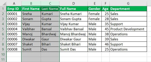
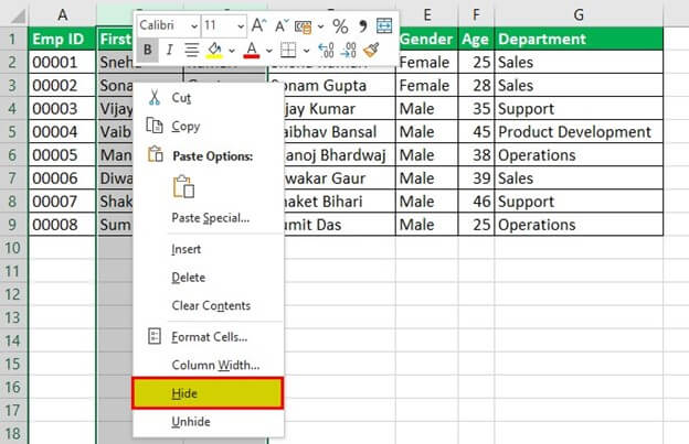
Right-click the selection and choose “hide” from the context menu. The same is shown in the following image.
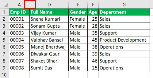
The final dataset, with columns B and C hidden, is shown in the following image. Notice that there are double vertical lines (shown in a red box) between the column labels A and D. These lines indicate that columns B and C have been hidden.

Another indication of hidden excel columns is the change in the sequence of the column labels. After label A, labels B and C are skipped, and straightaway label D is displayed.

Example #2–Hide Excel Columns Using the “Ctrl+Zero (0)” Shortcut

The following image shows a dataset similar to that of example #1. Notice that the number of columns has been reduced this time. Columns A to D are displayed, which consist of the employee ID, first name, last name, and full name respectively.

Ignore the green triangles in column A of the subsequent images. These are displayed because the “ignore error” option from the “trace error” button has not been clicked, unlike in step 1 of the preceding example (example #1).

We want to hide columns B and C by using the shortcut “Ctrl+zero (0)” in Excel.

The steps to hide the stated columns using the given technique are listed as follows:

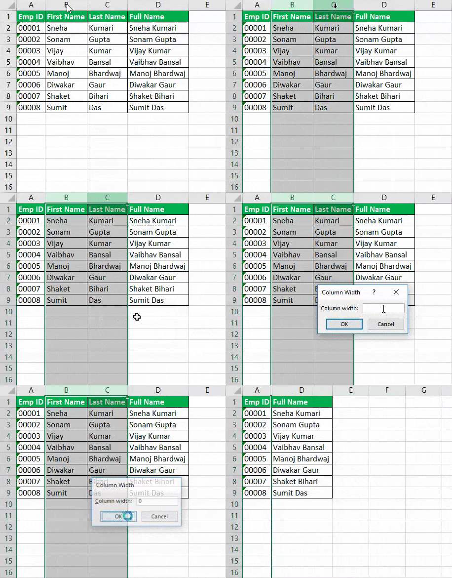
Step 1: Select columns B and C, which need to be hidden. For this, click the label of column B with the mouse and drag it across to column C. When the mouse pointer is placed on the label of column B, it changes to an arrow pointing downwards.

Note: Alternatively, select any cell of column B and press the keys “Ctrl+space” together. Column B is selected entirely. Next, press the keys “Shift+right arrow” to select column C.

Step 2: Once the columns to be hidden (columns B and C) are selected, press the keys “Ctrl+zero (0)” together.

The steps 1 and 2 are shown in the following image. Hence, columns B and C (selected in step 1) are hidden. Notice that, in the final output, the double vertical lines separate the labels of columns A and D.

Example #3–Hide Excel Columns by Setting the Column Width as Zero

Working on the dataset of example #2, we want to hide columns B and C by setting the column width as zero.

The steps to hide the mentioned columns using the given technique are listed as follows:

Step 1: Select the columns to be hidden. So, select columns B and C entirely.

Step 2: Right-click the selection and choose “column width” from the context menu. Set column width as zero and click “Ok.”

Both steps 1 and 2 are shown in the following image. The final dataset, with columns B and C hidden, is also displayed in this image. Double vertical lines appear between the labels of columns A and D.

Note: When a column’s width is entered as zero, the column is hidden from the worksheet.

Example #4–Hide Columns Using VBA Code

Working on the dataset of example #1, we want to hide columns B and C with the help of a VBA code. Consider the dataset to be in “sheet1” of Excel.

The steps to hide columns using a VBA code are listed as follows:

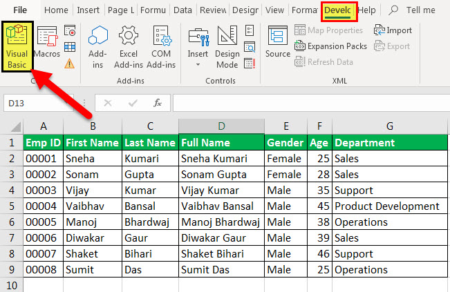
Step 1: From the Developer tab, click “visual basic.” This is shown in the following image.

Note: If the Developer tab is not displayed on the ribbon, it must be enabled from the File tab. For the detailed steps, click the given hyperlink.

Step 2: A new window titled “Microsoft visual basic for applications” opens. Double-click “sheet1.” Next, from the Insert tab, click “procedure.” Specify the name of the procedure and paste the following code:

Worksheets("Sheet1").Columns("B:C").Hidden = True

This is shown in the following image.

Step 3: Save the file with the .xlsm extension as it supports macros. This extension is used for a macro-enabled workbook, which has been created in Excel 2007 or the newer Excel versions.

Step 4: From the Run tab, click “run sub/user form.” The output is shown in the following image. Notice the double line (shown in a red box) between the column labels A and D. This indicates that the columns in between (i.e., columns B and C) are hidden.

Frequently Asked Questions

1. What does it mean to hide columns and how is it done in Excel?

To hide a column means removing one or more excel columns from the display. Such hidden columns do exist in the worksheet even though they become invisible. Columns are usually hidden when they are neither being used nor meant to be deleted.

The steps to hide a column in Excel are listed as follows:

a. Select the column to be hidden.
b. Right-click the selection and choose “hide” from the context menu.

The column selected in step “a” is hidden.

Note: For more techniques of hiding a column, refer to the examples of this article.

2. How to hide multiple columns in Excel?

The steps to hide multiple columns in Excel are listed as follows:

a. Select all the columns that need to be hidden.
• For selecting multiple contiguous columns, drag across the column labels with the mouse. Alternatively, select the first column and press the keys “Shift+right arrow” to select columns on the right.
• For selecting multiple non-contiguous columns, click the first column label. Thereafter, hold the “Ctrl” key and click the other column labels.
b. From the Home tab, click the “format” drop-down in the “cells” group.
c. Under “visibility,” select “hide & unhide.” Next, choose “hide columns.”

The columns selected in step “a” are hidden.

3. How to hide and lock columns in Excel?

The steps to hide and lock columns in Excel are listed as follows:

a. Select the entire worksheet by pressing either the keys “Ctrl+A” or the “select all” button. The “select all” button is located at the top-left corner of the Excel worksheet.
b. Right-click the selection and choose “format cells” from the context menu. The “format cells” dialog box opens. Uncheck the “locked” option in the “protection” tab. Click “Ok.”
c. Select the columns to be hidden and locked. Open the “format cells” dialog box again and click the “protection” tab. Check the “locked” option and click “Ok.”
d. Hide the columns selected in the preceding step (step c). For this, keep the columns to be hidden selected and click the “format” drop-down from the Home tab. Next, click “hide columns” from the “hide & unhide” option.
e. From the Review tab, click “protect sheet.” The “protect sheet” dialog box opens. Keep the following checkboxes selected:
• “Protect worksheet and contents of locked cell”
• “Select locked cells”
• “Select unlocked cells”
f. Enter a password and confirm it. Click “Ok” to proceed. The “protect sheet” dialog box closes.

The columns selected in step “c” are hidden. Since the worksheet is protected, these hidden columns cannot be unhidden by the usual ways to unhide a column. The advantage of locking hidden columns is that their content is concealed from the other users of the worksheet.

Note: To unhide the hidden columns, unprotect the sheet in the first place. To unprotect the sheet, click “unprotect sheet” from the Review tab. Next, enter the password and click “Ok.”

Thereafter, unhide the columns by selecting, right-clicking, and choosing “unhide” from the context menu. Alternatively, select the columns and choose “unhide columns” from the “hide & unhide” option of the “format” drop-down (in the Home tab).