ISERROR Excel Function

Last Updated :

21 Aug, 2024

Blog Author :

Edited by :

Reviewed by :

Table Of Contents

ISERROR Function in Excel

ISERROR is a logical function that is used to identify whether the cells being referred to have an error or not. This function identifies all the mistakes. If any error is found in the cell, it returns "TRUE" as a result, and if the cell has no errors, it gives "FALSE" as a result. This function takes a cell reference as an argument.

ISERROR function in Excel checks if any given expression returns an error in Excel.

For example, suppose you have a dataset and applied the ISERROR formula to divide the number by 0. In such a scenario, the ISERROR Excel function verifies the value and returns " TRUE" if it possesses an error. Therefore, Excel displays the #DIV/0! Error. Conversely, as a result, it provides " FALSE" if it does not consist of any error.

ISERROR Function in Excel

ISERROR Formula in Excel

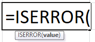
Arguments used for ISERROR Function.

Value: The expression or value to be tested for error.

The value can be a number, text, mathematical operation, or expression.

Returns

The output of ISERROR in Excel is a logical expression. If the supplied argument gives an error in Excel, it returns "TRUE." Otherwise, it returns "FALSE." For error messages- #N/A, #VALUE!, #REF!, #DIV/0!, #NUM!, #NAME?, and #NULL! generated by Excel, the function returns "TRUE."

ISERROR in Excel - Illustration

Suppose we want to see if a number gives an error when divided by another number.

We know that a number, when divided by zero, gives an error in Excel. Let us check if 21/0 provides an error using the ISERROR in Excel. To do this, we must type the syntax:

= ISERROR ( 21/0 )

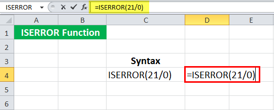
Press the "Enter" key.

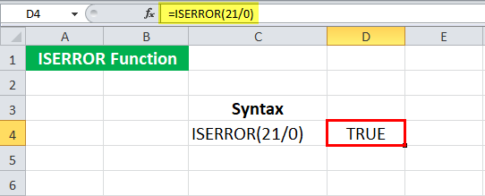
It returns "TRUE."

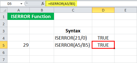
We can also refer to cell references in the ISERROR in Excel. Let us now check what will happen when we divide one cell by an empty cell.

When we enter the syntax:
= ISERROR ( A5/B5 )
Given that B5 is an empty cell.

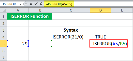
The ISERROR in Excel will return "TRUE."

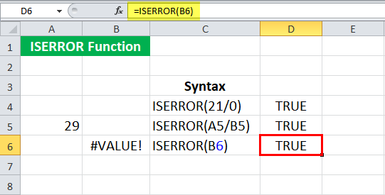
We can also check if any cell contains an error message. Suppose cell B6 has #VALUE! Which is an error in Excel. We may directly input the cell reference in the ISERROR in Excel to check if there is an error message or not as:

= ISERROR ( B6 )

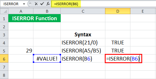
The ISERROR function in Excel will return "TRUE."

Suppose we refer to an empty cell (B7 in this case) and use the following syntax:

= ISERROR (B7)

Press the "Enter" key.

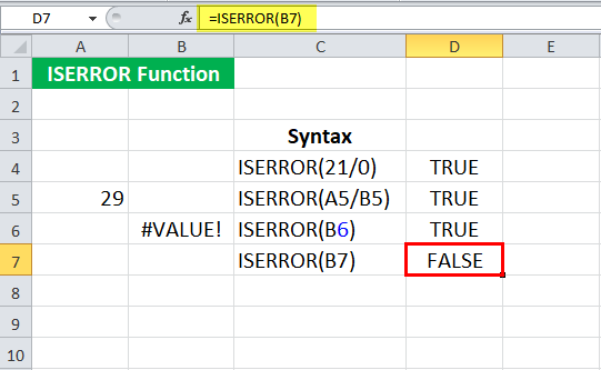
The ISERROR function in Excel may return "FALSE" since the Excel ISERROR function does not check for an empty cell. A blank cell is often considered zero in Excel. So, as we may have noticed above, if we refer to an empty cell in an operation such as division, it will be an error as it is trying to divide it by zero and thus returns "TRUE."

ISERROR Excel Function Video

How to Use the ISERROR Function in Excel?

The ISERROR function in Excel is used to identify cells containing an error. For example, there is often an occurrence of missing values in the data. If a further operation is carried out on such cells, the Excel may get an error. Similarly, if we divide any number by zero, it returns an error. Such errors further intervene if any other operation is carried out on these cells. In such cases, we can first check if there is an error in the operation. If yes, we can choose not to include such cells or modify the operation later.

ISERROR in Excel Example #1

Suppose we have the actual and forecast values of an experiment. The values are given in cells B4: C15.

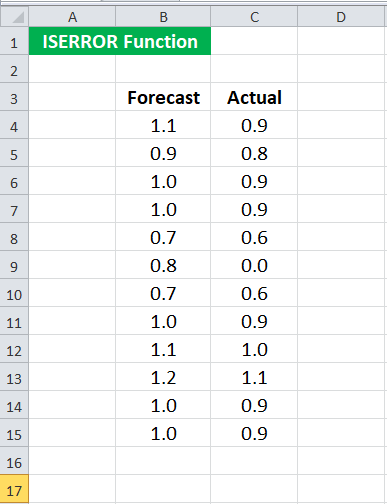
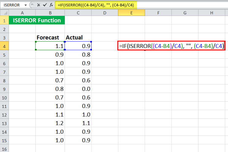
We want to calculate the error rate in this experiment, which is given as (Actual – Forecast) / Actual. However, we also know that some of the actual values are zero, and the error rate for such actual values will give an error. Therefore, we have decided to calculate the error for only those experiments which do not provide an error. To do this, we may use the following syntax for the first set of values:

We apply the ISERROR formula in Excel = IF( ISERROR ( (C4-B4) / C4 ), “” , (C4-B4) / C4)

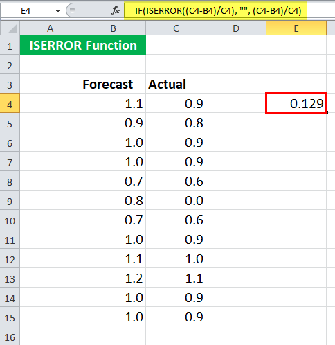
Since the first experimental values do not have any error in calculating the error rate, it will return the error rate.

We will get -0.129

You may now drag it to the rest of the cells.

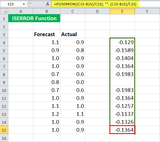
We will realize that the syntax returns no value when the actual value is zero (cell C9).

Now, let us see the syntax in detail.

= IF( ISERROR ( (C4-B4) / C4 ), “” , (C4-B4) / C4 )

ISERROR ( (C4-B4) / C4 ) will check if the mathematical operation (C4-B4) / C4 gives an error. In this case, it will return "FALSE."
If (ISERROR ( (C4-B4) / C4 ) ) returns "TRUE," the IF function will not return anything.
If (ISERROR ( (C4-B4) / C4 ) ) returns "FALSE," the IF function will return (C4-B4) / C4.

ISERROR in Excel Example #2

Suppose we are given some data in B4:B10. Some of the cells contain errors.

We want to check how many cells right from B4: B10 have an error. To do this, we may use the following ISERROR formula in Excel:

= SUMPRODUCT ( — ISERROR ( B4:B10 ) )

And press the "Enter" key.

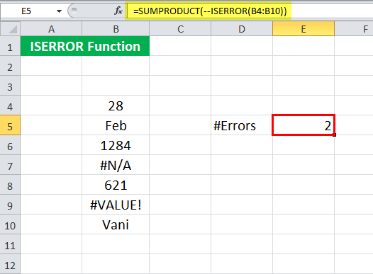
ISERROR in Excel will return 2 as there are two errors, i.e., #N/A and #VALUE!.

Let us see the syntax in detail:

ISERROR ( B4:B10 ) will look for errors in B4:B10 and return an array of TRUE or FALSE. Here, it will return {FALSE; FALSE; FALSE; TRUE; FALSE; TRUE; FALSE}
— ISERROR ( B4:B10 ) will then coerce TRUE/ FALSE to 0 and 1. It will return {0; 0; 0; 1; 0; 1; 0}
SUMPRODUCT (– ISERROR ( B4:B10 ) ) will then sum {0; 0; 0; 1; 0; 1; 0} and return 2.

ISERROR in Excel Example #3

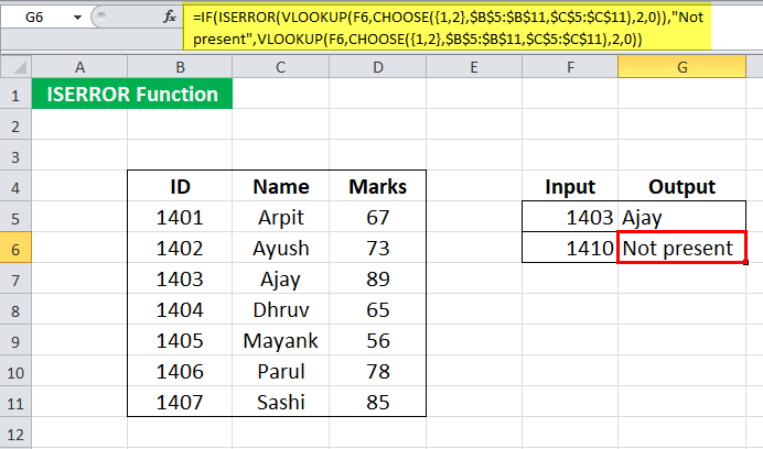
Suppose we have the enrollment ID, name, and marks of students enrolled in the course, given in cells B5:D11.

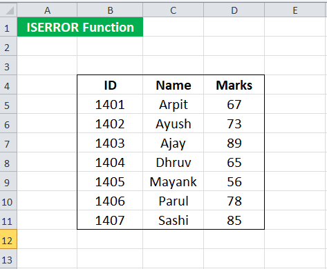
We must search for the student name given its enrollment ID several times. Now, we want to make the search easier by writing a syntax such that:

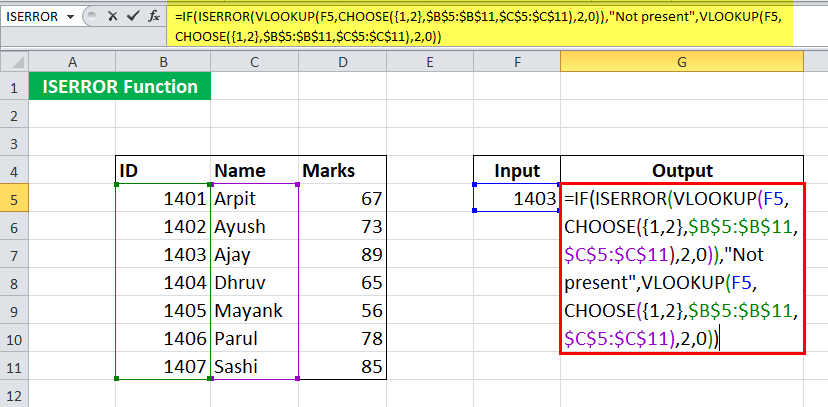
For any given ID, it should be able to give the corresponding name. Sometimes, the enrollment ID may not be present on the list. In such cases, it should return “Not found.” We can do this by using the ISERROR formula in Excel:

= IF( ISERROR( VLOOKUP( F5, CHOOSE( {1,2}, $B$5:$B$11, $C$5:$C$11 ) , 2, 0) ), “Not present”, VLOOKUP( F5, CHOOSE( {1,2}, $B$5:$B$11, $C$5:$C$11 ), 2, 0) )

Let us look at the ISERROR formula in Excel first:

CHOOSE( {1,2}, $B$5:$B$11, $C$5:$C$11 ) will make an array and return {1401,”Arpit”; 1402, “Ayush”; 1403, “Ajay”; 1404, “Dhruv”; 1405, “Mayank”; 1406, “Parul”; 1407, “Sashi”}
VLOOKUP( F5, CHOOSE( {1,2}, $B$5:$B$11, $C$5:$C$11 ) , 2, 0) ) will then look for F5 in the array and return its 2^nd
ISERROR( VLOOKUP( F5, CHOOSE(..) ) will check if there is an error in the function and return TRUE or FALSE.
IF (ISERROR( VLOOKUP( F5, CHOOSE(..) ), “Not present,” VLOOKUP( F5, CHOOSE() )) will return the corresponding name of the student if present. Else it will return “Not present.”

Use the ISERROR formula in Excel For 1403 in cell F5.

It will return the name “Ajay.”

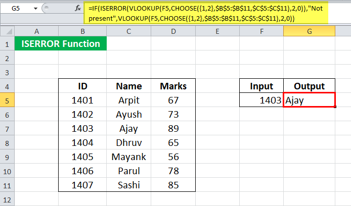
For 1410, the syntax will return “Not present.”

Things to Know about the ISERROR Function in Excel

The ISERROR function in Excel checks if any given expression returns an error.
It returns logical values, "TRUE" or "FALSE."
It tests for #N/A, #VALUE!, #REF!, #DIV/0!, #NUM!, #NAME?, and #NULL!.