Table Of Contents
What is "Not Equal To" Sign in Excel?
The “not equal to” is a logical operator in excel that helps compare two numerical or textual values. It is written (like <>) using a pair of angle brackets pointing away from each other. The “not equal to” excel sign returns either of the two Boolean values (true and false) as the outcome
- True implies that the two compared values are different or not equal.
- False implies that the two compared values are the same or equal.
For example, “=2<>4” (ignore the double quotation marks) returns “true” since the numbers 2 and 4 are not equal to each other.
The “not equal to” is used in the arguments of several Excel functions. The purpose of using the “not equal to” is to assess whether two values are different or not. However, the magnitude of difference is not conveyed by this operator.
How is the “Not Equal To” Sign Used in Excel?
Let us consider some examples to understand the working of the “not equal to” operator in Excel.
Example #1–Compare two Numeric Values with the “Not Equal To” Operator
The succeeding image shows the marks of students A and B (columns A and B) in 10 subjects. The total marks of each subject are 200. We want to find those rows for which the marks of the two students are unequal. Use the “not equal to” signof Excel.
The steps to find if a difference exists between the two marks are listed as follows:
Step 1: In cell C3, type the “equal to” symbol followed by the cell reference B3. Since the difference between cells B3 and A3 needs to be assessed, insert the “not equal to” sign between these two cell references.
The formula should look like the expression “=B3<>A3.” This expression is also known as a statement or a condition.
Note: A condition in Excel is an expression that evaluates to either true or false. At a given time, a condition cannot be assessed as both true and false.
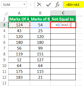
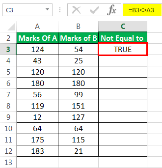
Step 2: Press the “Enter” key. The output in cell C3 is “true.” This is shown in the following image.
Step 3: Drag the formula of cell C3 till cell C12 by using the fill handle. This is shown in the following image.
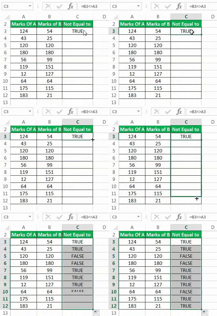
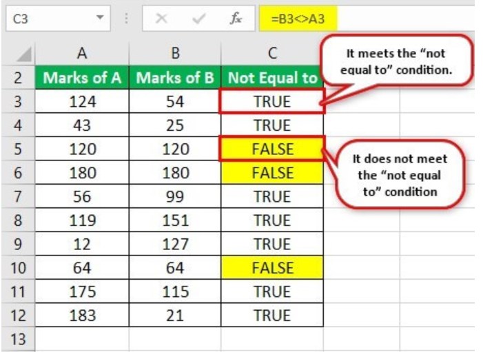
Step 4: The outputs for the entire column C are shown in the following image. The outputs which are false have been colored yellow. The inferences from this dataset are stated as follows:
- If the output is “true,” the values of column A and column B for a given row are not equal. This means that the “not equal to” excel condition for that particular row is met. For instance, the “not equal to” condition for row 3 is “=B3<>A3.” In other words, 124 is not equal to 54.
- If the output is “false,” the values of column A and column B for a given row are equal. This means that the “not equal to” condition for that particular row is not met. For instance, the “not equal to” condition for row 5 is “=B5<>A5.” In other words, 120 is certainly equal to 120.
Overall, for three rows (rows 5, 6, and 10), the marks of students A and B are equal. Except for these rows, the marks are unequal in all the remaining rows (rows 3, 4, 7, 8, 9, 11, and 12). Without knowing the magnitude of difference, one cannot conclude whose performance (from students A and B) is better.
Example #2–Compare two Textual Values with the “Not Equal To” Operator
In the dataset of example #1, we have substituted random grades (from A to J) in place of numbers. We want to find the rows for which the grades of students A and B are unequal. Use the “not equal to” operator of Excel.
The steps to find if a difference exists (between the grades) are listed as follows:
Step 1: Enter the formula “=B3<>A3” in cell C3. Press the “Enter” key. The output in cell C3 is “true.” So, for row 3, the “not equal to” excel operator has validated that the values in the first and second cell (A3 and B3) are not equal.
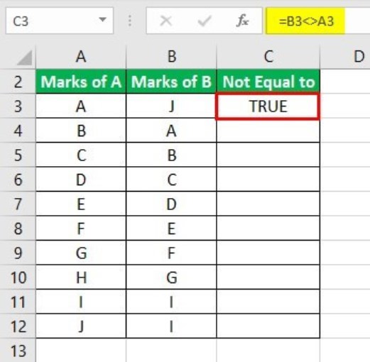
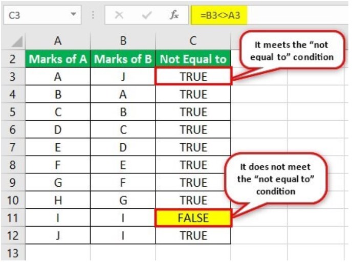
Step 2: Drag the formula of cell C3 till cell C12. The outputs for the entire column C are shown in the following image. The single false output has been colored yellow.
The output in cell C3 meets the “not equal to” excel condition, which is “=B3<>A3.” In contrast, the output in cell C11 does not meet the “not equal to” condition, which is “=B11<>A11.” Hence, the grades of all rows, except row 11, are unequal. The grades of the two students are equal for row 11.
Example #3–Obtain Defined Results with the IF Function and the “Not Equal To” Condition
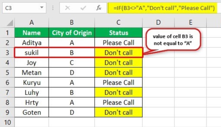
The succeeding image shows the names of a few candidates and their native places in columns A and B respectively. From these candidates, an organization wants to hire those candidates whose city of origin is “A.”
We want to differentiate candidates who need to be contacted and who need not be contacted for the further hiring process. For this, display the status as either “please call” or “don’t call” (in column C), depending on whether the hometown of a candidate is “A” or not.
Use the IF function and the “not equal to” operator of Excel.
The steps to use the IF function and the “not equal to” operator are listed as follows:
Step 1: Enter the following formula in cell C2.
“=IF(B2<>"A","Don’t call","Please Call")”
Press the “Enter” key. Drag the formula till cell C9. The outputs of column C are shown in the succeeding image. The candidates whose city of origin is “A” have been assigned the “please call” status in column C.
Note: In the given IF formula, the condition is the logical test. The string “don’t call” is “value_if_true” and the string “please call” is “value_if_false.”
So, the IF formula returns “don’t” call” for a given row, if the value of column B is not equal to “A” (i.e., the condition is true). It returns “please call” for a given row, if the value of column B is equal to “A” (i.e., the condition is false).
With the help of the IF function, Excel can display different results for the matched and unmatched conditions. For more details related to the IF function of Excel, click the hyperlink given immediately before step 1 of this example.
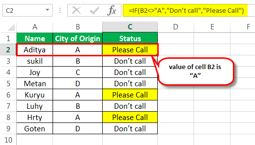
Step 2: The candidates whose hometown is other than “A” have been assigned the “don’t call” status in column C. This is shown in the following image.
Hence, only candidates “Aditya,” “Kuryu,” and “Hrty” should be called for the further round of interviews. The remaining candidates need not be contacted.
So, with the IF function and the “not equal to” excel operator, we have successfully differentiated the candidates who can be hired from those who cannot be hired.
Note: Notice that this step has been added only for the purpose of understanding. The preceding step (step 1) is complete in itself for the given task of hiring candidates.
Example #4–Count Specific Cells with the COUNTIF Function and the “Not Equal To” Condition
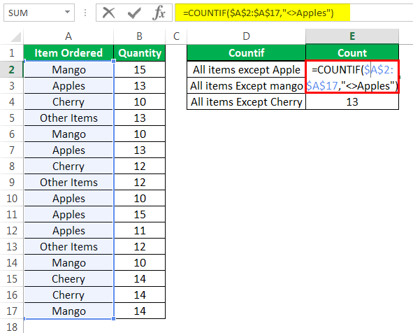
The succeeding image shows certain fruits (or items) in column A and their quantities ordered in column B. Apart from apples, mangoes, and cherries, the remaining fruits have been clubbed under “other items” in column A.
We want to count the number of cells (of column A) that are not equal to:
- “Apples”
- “Mango”
- “Cherry”
There should be three outputs, one output excluding one fruit. Use the COUNTIF function and the “not equal to” operator of Excel.
The steps to use the COUNTIF function and the “not equal to” operator are listed as follows:
Step 1: Enter the following formulas in cells E2, E3, and E4 respectively.
- “=COUNTIF($A$2:$A$17,"<>Apples")”
- “=COUNTIF($A$2:$A$17,"<>Mango")”
- “=COUNTIF($A$2:$A$17,"<>Cherry")”
Press the “Enter” key after entering each formula.
The first formula counts the number of cells in the range A2:A17, which do not contain the string “apples.” Likewise, the second formula counts the number of cells in this range that do not contain the string “mango.” The third formula helps count the number of cells in the given range (A2:A7), which do not contain the string “cherry.”
Notice that the succeeding image shows the formula in cell E2 and the result of the third formula in cell E4.
Note: “$A$2:$A$17” is the “range” argument of the preceding COUNTIF formulas. The condition "<>Apples" is the “criteria” argument of the first formula. In all the preceding formulas, the range is the same, but the criterions are different.
The COUNTIF counts the cells of a range, which satisfy a single criterion. For more details related to the COUNTIF function, click the hyperlink given before step 1 of this example.
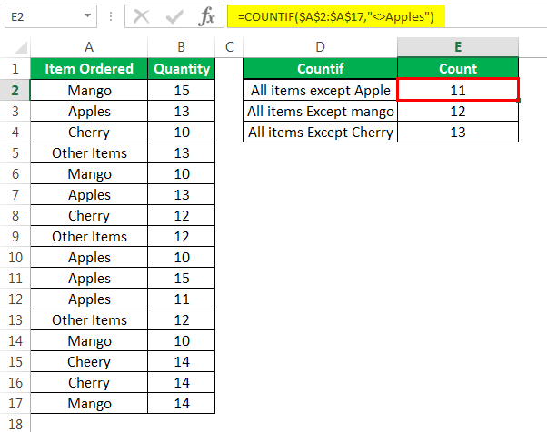
Step 2: The following image shows the three outputs (in cells E2, E3, and E4) of the three formulas entered in the preceding step.
Notice that “cherry” has been deliberately misspelled as “cheery” in cell A15. As a result, this cell has also been counted (as a cell not containing “cherry”) by the third COUNTIF formula.
Had the word been correctly spelled in cell A15, the output in cell E4 would have been 12. In this case, cell A15 would have been excluded from the count (as a cell containing “cherry”).
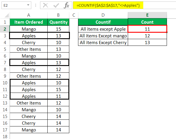
Step 3: The rows containing “apples” are displayed in black boxes in the following image. These rows are excluded while counting the cells not containing “apples.” Hence, 11 cells (in the range A2:A17) do not contain the string “apples.”
Likewise, in the given range, 12 cells do not contain the string “mango” and 13 cells do not contain the string “cherry.”
Note: This step has been added only for notifying the readers, the cells that are counted and the cells that are left out by the first COUNTIF formula (entered in step 1).
Example #5–Sum Particular Cells with the SUMIF Function and the “Not Equal To” Condition
Working on the data of example #3, we want to sum the quantities of column B that are not equal to:
- “Apples”
- “Mango”
- “Cherry”
There should be three summed outputs where each output excludes one fruit. Use the SUMIF function and the “not equal to” sign of Excel.
The steps to use the SUMIF function and the “not equal to” operator are listed as follows:
Step 1: Enter the following formulas in cells E2, E3, and E4 respectively.
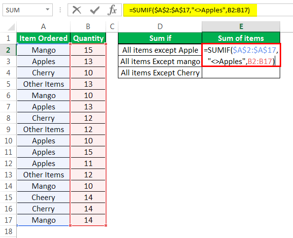
- “=SUMIF($A$2:$A$17,"<>Apples",B2:B17)”
- “=SUMIF($A$2:$A$17,"<>Mango",B2:B17)”
- “=SUMIF($A$2:$A$17,"<>Cherry",B2:B17)”
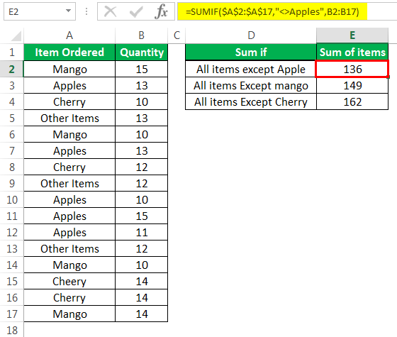
The first formula is shown in the following image.
In all three formulas, the SUMIF function evaluates the range A2:A17. For cells not equal to “apples” (in range A2:A17), the first formula sums the numbers of the range B2:B17. Likewise, for cells not equal to “mango” in the given range (A2:A17), the second formula also sums the numbers of the range B2:B17. Similar summing is carried out by excluding cells containing “cherry.”
Note: “$A$2:$A$17” is the “range” argument of the SUMIF function. The condition "<>Apples" is the “criteria” argument. The range “B2:B17” is the “sum_range” argument of the SUMIF function.
With the SUMIF function, we have applied the given condition (in each formula) to the range A2:A17 and summed up the corresponding values of the range B2:B17. Usually, the SUMIF works with a single criterion. For more details related to the SUMIF function, click the hyperlink given before step 1 of this example.
Step 2: Press the “Enter” key after entering each of the preceding formulas. The three summed outputs are shown in the following image.
Hence, the sum of all the fruit quantities except “apples” is 136. Excluding the cells containing “mango,” this sum is 149. Likewise, leaving the cells containing “cherry,” this sum is 162.
Notice that the value of cell B15 has also been included in the sum returned (in cell E4) by the third SUMIF formula (entered in step 1). This is because in cell A15, the spelling of “cherry” has been misspelled as “cheery.” Hence, Excel considers A15 as a cell not containing “cherry.”
