


What Is A Jump Diffusion Model?
A jump diffusion model refers to a stochastic volatility framework used in quantitative finance to gauge the unexpected movement in asset prices, whether upwards or downwards. It, thus, coincides with the space-time Poisson model’s lognormal jump component with the geometric Brownian motion’s diffusion component for asset pricing and hedging.
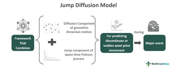
Merton’s jump diffusion model finds a place in predicting stock price volatility when the market is facing hardship amidst a significant economic crisis, pandemic, war, or other such events. In such scenarios, the asset prices increase or decrease in a discontinuous pattern (jump or shock), therefore necessitating the use of both jump and diffusion components.
Key Takeaways
- A jump diffusion model refers to a hybrid framework in stochastic volatility predictive analysis that emphasizes on combining the lognormal jump component derived from the space-time
- Poisson process with the diffusion element of the geometric Brownian motion to predict discontinuous fluctuation in asset prices during significant event or market conditions.
- It overcomes the pitfalls of the Black Scholes model that assumes a lognormal distribution of returns even when a significant event influences the market.
- This framework was developed by the American economist Robert C. Merton in 1976.
Jump Diffusion Model in Finance Explained
The jump diffusion model is an integrated version of the two fundamental processes of stochastic volatility predictions, I.e., jump and diffusion. The jump component here signifies the lognormal jump acquired from the space-time Poisson process and the diffusion element from the well-known geometric Brownian motion.
It is a widely used framework to address the pitfalls of the Black-Scholes model that fails to consider that asset returns usually have thick tails.
In this process, the diffusion component studies the continuous fluctuations in the asset prices that either fall or rise gradually over the period. At the same time, the jump factor considers any sudden or unexpected price movement (shocks or jumps) in stocks due to a specific market change or event. Thus, it provides a complete overview of the asset price changes in the market, whether regular or irregular, fostering informed decision-making and risk management related to asset pricing and hedging.
In 1976, an American economist, Robert C. Merton, discovered that asset prices don’t show a continuous or consistent movement during a significant occurrence like a pandemic, economic crisis, or war. Moreover, he believed that in such circumstances, two different models influence stock prices, the Poisson process and the Brownian motion, resulting in the foundation of Merton’s jump diffusion model.
Finance Applications
Merton’s jump diffusion model is a hybrid framework that allows for a comprehensive analysis of stock pricing even when the market is affected by any substantial happenings. Let us now discuss its various implications in finance:
- Gauging Discontinuous Asset Pricing Behavior: When the market experiences sudden upswings or downfalls due to significant events like war, pandemic, or economic distress, this model helps to identify such discontinuous movement in asset prices.
- Pricing of Options: Double exponential jump diffusion model for options pricing facilitates articulating the various options pricing problems such as interest rate derivatives, call and put options, and path-dependence options.
- Hedging: In European options, it becomes crucial to mitigate the quadratic risk potential at maturity through hedging, which can be determined through this framework.
- Credit Risk Modelling: This hybrid model helps in pricing risky assets or debt instruments like convertible bonds by using the probability distribution of the default jump function.
- Predicting Real Estate Market: In real estate, such frameworks help to estimate the future value of the properties based on various real estate factors like size, location, use, etc.
- Optimizing Portfolio: Fund managers often use jump diffusion frameworks for asset price predictions to develop strategies that mitigate risk and maximize returns to investors.
Examples
Financial market analysts and traders widely use jump diffusion models to devise pricing solutions in the financial markets. Below are some of the relevant examples:
Example #1
Suppose Mr. A and Mrs. B are the financial market analysts. Mr. A determines the asset prices using the Black-Scholes model, and Mrs. B employs the jump diffusion model to predict the asset prices. Now, in a scenario where the market showed discontinuous asset price fluctuations during the COVID-19 pandemic, Mrs. B was able to predict a sharp fall in the S&P 500 and, therefore, purchased a covered call put option based on the prediction of a decline in its options pricing. She, thus, made a profit even in the adverse market conditions. At the same time, Mr. A was unable to spot any such opportunity.
Example #2
The liberalization of European gas markets led to a fragmented supply chain, introducing residual shape risk (RSR) due to inadequate hedging granularity. RSR is, therefore, a subclass of commodity risk that reflects the difference between forward and spot gas prices weighted by volume deviation. It thus emphasizes the empirical analysis of the Czech gas market by employing volumetric hedging that utilized the OTE price index as spot price data.
This shift towards financial market practices necessitates risk metrics like Value-at-Risk (VaR) and Expected Shortfall (ES). A prominent risk management strategy to address the market’s complexity, including factors like jumps, volatility, and mean reversion, is the use of jump diffusion models.
Source – https://www.sciencedirect.com/science/article/abs/pii/S0140988319302464
Advantages And Disadvantages
Although jump diffusion models are more effective for interpreting stochastic volatility when compared with the Black-Scholes model, they have been developed further to overcome their potential limitations. Let us now discuss the various pros and cons of this framework below:
| Advantages | Disadvantages |
|---|---|
| The jump diffusion model provides more reliable results by considering the shocks or jumps pertaining to the sudden, unexpected, or discontinuous changes in asset prices during significant occurrences. | Being a hybrid model, it requires the collection of considerable data to derive reliable outcomes, which can be challenging for market analysts, researchers, and traders. |
| Since it considers both the jump and diffusion components, it is able to anticipate future asset pricing more accurately. | Unlike the Black Scholes model, the jump diffusion framework is quite complex in its implementation and calibration and may involve errors if not used effectively. |
| The model is highly adaptable and flexible to incorporate significant market changes by considering jumps or shocks with varying frequency or intensity. | Its computation is complex and time-consuming due to the consideration of various parameters based on the current market data, especially in rigid market scenarios. |
| It facilitates options pricing, hedging, and credit risk modeling in the financial markets. |
Frequently Asked Questions (FAQs)
Frequently Asked Questions
What is the difference between jump diffusion models for option pricing and the Black Scholes model?
The jump diffusion model provides more reliable outcomes in asset pricing, since, it doesn’t assume lognormal distribution of returns, unlike the Black-Scholes model.
What is the formula for the jump diffusion model?
The stochastic volatility jump diffusion model formula: dSt=tStdt+tStdWt+UtStdNt; here, – μt and σt represent the time deterministic functions; – Wt denotes the Brownian motion; – Nt is the space-time Poisson process comprising parameter λ, independent of Wt; – Ut indicates the jump component, which is S’s relative jumping strength denoted as: Uj=[Sj-Sˉj]Sˉj; where, j denotes the jth stay time.
What is the primary feature of a jump diffusion model?
The jump diffusion model has a leptokurtic feature in contrast to the normal distribution of returns; the asset prices may touch the high peak with heavy asymmetric tails.