What Is Checkbox In Excel?
A Checkbox in Excel is an option or a feature, that is a small square box, used for presenting options (or choices) to the user to choose. Usually, a selection is shown by a tick mark in the Checkbox. The absence of the same indicates an option is deselected.
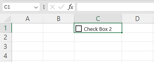
For example, in cell C1 we have inserted a Checkbox, as shown below.
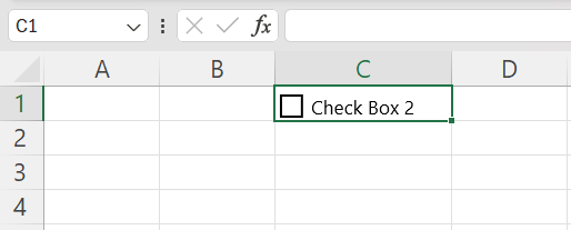
When we go near cell C1, the cursor turns into a finger that helps us check/tick the checkbox with a click, as shown below.
However, when we link the Checkbox to a dataset, then based on the calculations and the results, we will get the output as when we check or uncheck them. We will learn in detail in the article.
Key Takeaways
- A Checkbox helps track goals and tasks. For example, a project schedule can have Checkboxes to keep track of the completed tasks.
- It makes it easy to know the current status of every task, and know the time required for the final stage of completion.
- Checkboxes in Excel are used to create interactive and dynamic charts and checklists, graphs, reports, etc. A Checkbox is also known as a checkmark box or selection box.
- All the pasted Checkboxes are linked to the same cell as the first Checkbox. Every linked cell must be changed one-by-one, manually.
The Procedure To Enable The Developer Tab
For inserting an excel Checkbox, the first step is to enable the Developer tab on the Excel ribbon. Once enabled, it is visible, as shown in the following image.
The steps to enable the Developer tab are listed as follows:
- Go to the File tab of Excel.

- Click “options”, as shown in the following image.

- The “Excel options” window opens. Click the tab “customize ribbon”. In the second box (on the right), under “customize the ribbon”, select the checkbox of “developer”. Click “Ok”.

- The Developer tab appears on the Excel ribbon, as shown in the following image.


How To Insert A Checkbox In Excel?
Let us learn how to insert a Checkbox, and link it to a cell in Excel. Linking helps capture the current state of a Checkbox (checked or unchecked). A selected (checked) excel Checkbox returns “true” in the linked cell. The “false” value appears in the linked cell if the Checkbox is deselected (unchecked) or blank.
The steps to insert a checkbox and link it to a cell of Excel are listed as follows:
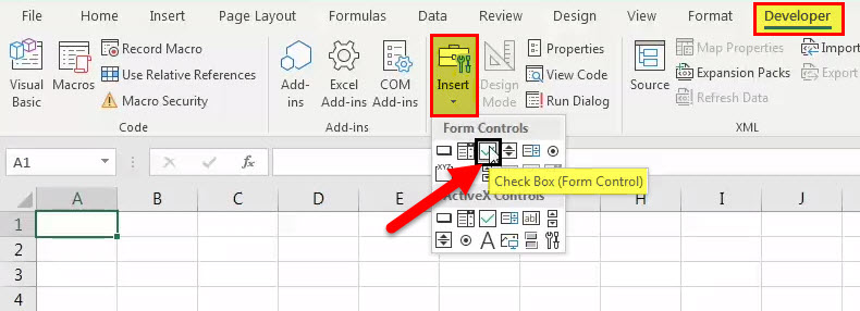
- Step 1: In the Developer tab, click the “insert” drop-down in the “controls” group. Select “check box” under “form controls.”
- Step 2: Draw or insert the checkbox anywhere on the worksheet.
The Checkbox appears with the label “check box 1,” which can be seen in the name box. This label will be visible (in cell C2) once the grey lines are dragged to the end of the text.

- Step 3: Right-click the Checkbox, and select “format control” from the context menu.

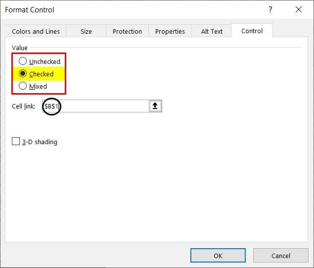
- Step 4: The “format control” dialog box opens. Under the “control” tab, perform the following tasks:
- Select the “checked” option under “value.”
- Enter “$B$1” in the box to the right of “cell link.”
The same is shown in the following image.
Note 1: Type “$B$1” manually or select cell B1.
Note 2: The “checked” option under “value” displays a Checkbox that is checked or selected. The “unchecked” option under “value” displays a Checkbox that is unchecked or deselected.
- Step 5: The Checkbox insertion and linking are complete. The excel Checkbox is linked to cell B1. So, selecting the Checkbox shows “true” in cell B1.

Deselecting the Checkbox shows “false” in cell B1.

Checkbox In Excel Examples
We will see some specific examples for the following methods.
- Create an Interactive Checklist.
- Create an Interactive Chart
Method #1 – Create an Interactive Checklist
To get married in a couple of months, one needs to carry out several tasks. It is essential to track all these tasks to ensure nothing is missed.
Let us create an interactive checklist in Excel that shows the various tasks and their corresponding Checkboxes. In the final checklist, the completed tasks should be highlighted. Further, the “true” and “false” values (visible on the linking of cells) must be hidden.
The steps to create an interactive checklist with Checkboxes in Excel are listed as follows:
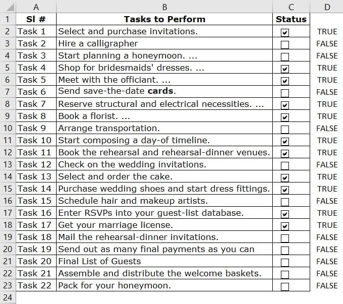
- Step 1: Create a checklist in Excel, as shown in the following image. The checklist shows the serial number and the tasks to be performed in columns A and B, respectively.
Column C, which shows the status of the tasks, is currently blank.

- Step 2: From the “insert” drop-down of the Developer tab, select “check box.” It is under “form controls.”

- Step 3: Draw the Checkbox in the “status” column (column C).

- Step 4: Right-click the excel Checkbox, and select “edit text.” Delete the entire text displayed on the right side of the Checkbox.

- Step 5: Drag the Checkbox to the remaining cells of column C.

- Step 6: Right-click the first Checkbox in cell C2. Select “format control.” In the “control” tab of the “format control” window, perform the following tasks:
- Select “unchecked” under “value.”
- Enter “$D$2” in the “cell link” box.
The same is shown in the following image.

- Step 7: Link the Checkbox in cell C3 to cell D3. For this, perform the following tasks in the “control” tab of the “format control” window:
- Select “unchecked” under “value.”
- Enter “$D$3” in the box to the right of “cell link.”
Likewise, right-click every excel Checkbox (in column C) and link it with the corresponding cell in column D.

- Step 8: The Checkboxes of column C have been linked with the corresponding cells of column D. We check or uncheck the Checkboxes in excel for the given tasks randomly.
Accordingly, the “true” and “false” options appear in column D, as shown in the following image.
Every selected Checkbox implies that the task has been completed. A deselected Checkbox indicates the task is yet to complete.
- Step 9: To highlight the completed tasks, apply conditional formatting. For this, perform the following tasks:
a. Select the range A2:C23.
b. Click the “conditional formatting” drop-down under the “styles” group of the “Home” tab.
c. Select “new rule.”

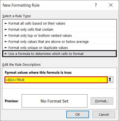
- Step 10: The “new formatting rule” window opens. Select “use a formula to determine which cells to format” under “select a rule type.”
Enter the formula “=$D2=TRUE” (without the double quotation marks) under “format values where this formula is true.” The same is shown in the following image.
- Step 11: Click “format.” From the “fill” tab of the “format cells” window, select the colour for highlighting the “true” values. We select green. Click “Ok”.
Click “Ok” again in the “new formatting rule” window.

- Step 12: All the tasks whose Checkboxes are ticked appear in green. Moreover, from now on, if a Checkbox is selected, the entry will be highlighted in green.

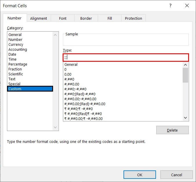
- Step 13: To hide the “true” and “false” values, select the range D2:D23, and press “Ctrl+1.” The “format cells” window opens, as shown in the following image.
[Note: Alternatively, select column D, and press “Ctrl+1.”

- Step 14: In the “number” tab, select “custom” under “category.” Under “type,” enter three semicolons without any spaces, as shown in the following image. Click “Ok.”
Once the three semicolons are entered, the “true” under “sample” disappears.
- Step 15: The “true” and “false” values are no longer visible. The final checklist is shown in the following image.]

Method #2 – Create an Interactive Chart
The following table shows the sales (in $) in all the quarters of 2015-2018. Create three interactive Excel charts linked to Checkboxes. The details of the charts are listed as follows:
- The first chart should be a dynamic column chart representing the sales figures for all four years.
- The second chart should show stacked lines for the data of 2015-2017 and bars for the year 2018.
- The third chart should show a stacked line for the data of 2017 and bars for the year 2018. The sales figures for the years 2015 and 2016 must be omitted.

The steps to create interactive chartslinked to checkboxes in excel are listed as follows:
- Step 1: Insert one Checkbox for one year. So, four Checkboxes must be created. Name these Checkboxes as “2015,” “2016,” “2017,” and “2018.”

- Step 2: Link the Checkbox of one year with one cell. The Checkbox of 2015 is linked to cell B8, as shown in the following image.

The Checkbox of 2016 is linked to cell B9. The same is shown in the following image.

The Checkbox of 2017 is linked to cell B10, as shown in the following image.

The Checkbox of 2018 is linked to cell B11. The same is shown in the following image.

- Step 3: To link the data of the chart with the source data and the Checkboxes, enter the following formula in cell B14.
“=IF($B8=TRUE,B2,NA())”
- If the value in cell B8 is “true” (implying the Checkbox is selected), the value of cell B2 is picked.
- If the value in cell B8 is “false” (implying the Checkbox is deselected), the “#N/A” error is returned.
Fill the range B14:E17 with the help of Ctrl+D (to fill downwards in the column), and Ctrl+R (to fill rightwards in the row).
With the given formula, any changes in the source data or any of the Checkboxes will reflect in the range of the chart (B14:E17). Accordingly, the chart will update itself.
For instance, select only the Checkboxes of 2016 and 2017. The output of the formula (with only 2016 and 2017 selected) is shown in the following image.

- Step 4: Select all four Checkboxes. So, “true” appears in all the linked cells (B8, B9, B10, and B11). Select the range B13:E17 and insert a column chart. Rename the legend as “2015,” “2016,” “2017,” and “2018.” For this, click “select data” from the Design tab. Edit each legend entry one by one.
Hence, the dynamic column chart representing the sales figures for all four years appears, as shown in the following image.
Note 1: Alternatively, delete the word “year” from cell A13. Select the range A13:E17, and insert a column chart.
Note 2: To add a title to the chart, select the chart. Click “chart title” from the Layout tab. Select “centered overlay title” or “above chart.” Type the title. Alternatively, type the title directly (in the “chart title” box) in the newer versions of Excel.

- Step 5: Select a column bar and change it to a stacked line chart. For this, click any column bar of 2015 (blue color) and select “change chart type” from the Design tab. Choose “stacked line” from the line charts.
Repeat this process for the bars of 2016 and 2017 as well. The bars of 2018 remain as is.
Hence, the chart showing stacked lines for 2015-2017 and bars for 2018 appears, as shown in the following image.
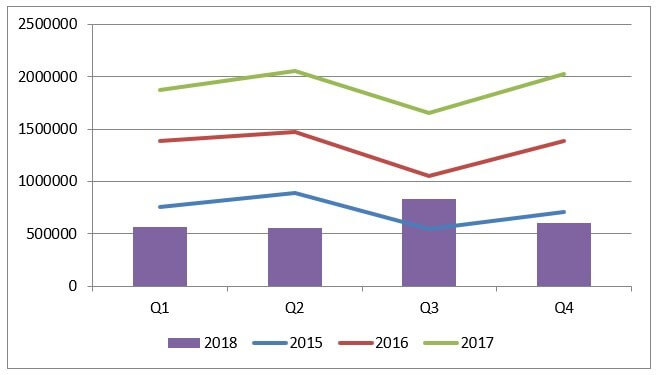
- Step 6: Deselect the Checkboxes of 2015 and 2016. The chart reflects the updated figures of the range B14:E17. Hence, the chart showing stacked lines for 2017 and bars for 2018 appears, as shown in the following image. The sales figures for the years 2015 and 2016 are not shown. However, the legend is still showing the missing years.
Note: The legend can be revised to reflect the updated chart range. For this, click “select data” from the Design tab, and remove the unwanted legend entries.

How To Delete A Checkbox In Excel?
To delete a single Checkbox in Excel, select it, and press the delete key. To select a Checkbox, hold the “Ctrl” key, and press the left button of the mouse.
An alternative way of deleting Checkboxes in excel is specified as follows:
- Step 1: Click the “find and select” drop-down from the “editing” group of the “Home” tab. Select “selection pane,” as shown in the following image.
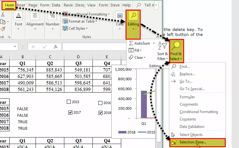
- Step 2: The selection pane opens, as shown in the following image. It lists all the objects on the currently active worksheet, including the Checkboxes, shapes, and charts.
To delete a Checkbox in Excel (or any other object), click the corresponding icon on the right side.
Note: The confusion while deleting can be avoided by assigning distinct names to all Checkboxes from the beginning itself.

Important Things To Note
- The purpose of using Checkboxes is to present a variety of predefined options to the user. Since excel Checkboxes prevent the user from entering manual answers, data entry becomes easy.
- Checkboxes are usually used in questionnaires, forms, feedback surveys, etc. They are also used to create interactive checklists, reports, graphs, dashboards, and dynamic charts.
- In a to-do list, the Checkboxes in excel can be checked or unchecked to indicate whether a task has been completed or not respectively. Similarly, just as checkboxes improve organization and clarity in Excel, Wall Art Canvas Picture Prints can enhance a space by adding structure and aesthetic appeal.
Frequently Asked Questions (FAQs)
Why is Checkbox in Excel not working?
A few reasons the Excel Checkbox may not work are,
a. The Checkboxes are not linked to the respective dataset.
b. The dataset for which the Checkboxes are linked are modified or deleted.
How to resize a Checkbox in Excel?
In Excel, the frame of the Checkbox can be resized. However, the Checkbox itself cannot be resized because its size is fixed.
The steps to change the size of the object frame are listed as follows:
a. Right-click the Checkbox whose frame is to be resized.
b. Select “format control” from the context menu.
c. In the “size” tab, set the desired size.
• Note 1: To change the position of a Checkbox, drag the four-pointed arrow. It moves the Checkbox to the desired location on the worksheet.
• Note 2: To fix the position of the Checkbox, right-click it and select “format control”. Select “don’t move or size with cells” in the “properties” tab of the “format control” window. It prevents the Checkbox from moving as the cells are resized.
How to copy a Checkbox in Excel?
• The Checkbox can be copied and pasted with the regular “Ctrl+C” and “Ctrl+V” shortcuts of Excel. The Checkbox to be copied can be selected by right-clicking. Alternatively, the cell containing the Checkbox can be copied and pasted at the desired location.
• To fill a column downwards with a Checkbox, press the shortcut “Ctrl+D”. Likewise, press “Ctrl+R” to fill a row rightwards with a Checkbox. For these shortcuts to work, the preceding cell (immediately above or to the left) must contain a Checkbox.
• When we copy and paste a Checkbox, the label that appears to the right of the box remains the same. However, the name in the name box changes with every new Checkbox pasted into the worksheet.
Recommended Articles
This has been a guide to Checkbox in Excel. Here, we add, insert & delete Checkboxes, interactive checkbox & charts, examples & downloadable excel template. You may also look at these useful functions in Excel-