Date Range In Excel

Date Range in Excel helps users find results based on data with dates. We need to perform different operations like addition or subtraction on date values with Excel. By setting date ranges in Excel, we can perform calculations on these dates. For setting date ranges in Excel, we can first format the cells that have a start and end date as ‘Date’ and then use the operators: ‘+’ or ‘-‘to determine the end date or range duration.

For example, suppose we have two dates in cells A2 and B2. To create a date range, we may use the following formula with the TEXT function:

=TEXT(A2,”mm/dd")&" - "&TEXT(B2,"mm/dd")

• For conducting date-related calculations in Excel, one must format cells with start and end dates as 'Date,' then use '+' or '-' to know the end date or range duration.
• To make a list of sequential dates in Excel, choose the starting date cell, pull it to the range you want to fill the dates, navigate to "Home" > "Editing" > "Fill Series," choose the date unit, and click "OK." The selected cells will be filled with sequential dates.
• To calculate the number of days between two dates, one can deduct the two dates utilizing the '-' operator.

Date Range in Excel is not an inbuilt formula. But, we can manually find the result with TEXT function.

So, the date range in Excel formula is,

=TEXT(A2,”mm/dd")&" - "&TEXT(B2,"mm/dd")

Now, let us learn how to use date range in Excel with detailed examples.

Example #1 - Basic Date Ranges

Let us see how adding a number to date can create a date range.

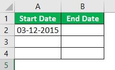
Suppose we have a start date in cell A2.

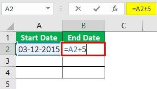
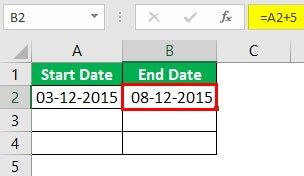
If we add a number, say 5, to it, we can build a date range.

When we select cell A3 and type “=B2 + 1.”

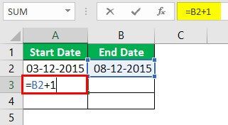
Then, we need to copy the cell B2 and paste it into cell B3; the relative cell reference would change as follows:

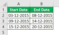
So we can see that multiple date ranges can be built this way.

Example #2 - Creating Date Sequence

With Excel, we can easily create several sequences. Now we know that dates are some numbers in Excel. So we can use the same method to generate date ranges. So to create date ranges that have the same range or gap, but the dates change as we go down, we can follow the below steps:

• We must first type a start date and end date in a minimum of two rows.

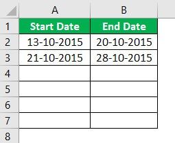
• Then, select the ranges and drag them down below the row where we require the dates ranges.

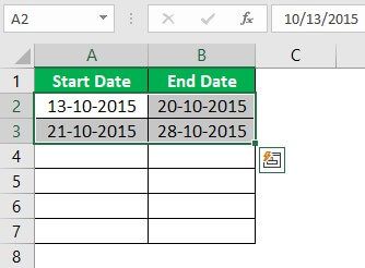
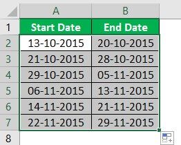
So we can see that using the date ranges in the first two rows as a template, Excel automatically creates date ranges for the subsequent rows.

Example #3

Now, suppose we have two dates in two cells, and we wish to display them concatenated as a date range in a single cell. For doing this, we can use a formula based on the TEXT function. The general syntax for this formula is as follows:

= TEXT(date1,”format”) & ” – ” & TEXT(date2,”format”)

Case 1:

This function receives two date values as numeric and concatenates these two dates in the form of a date range according to a custom date format (“mmm d” in this case):

Date Range =TEXT(A2,”mmm d”) & “-” & TEXT(B2,”mmm d”)

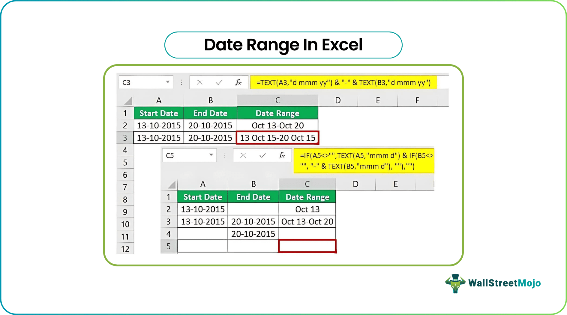
So we can see in the above screenshot that we have applied the formula in cell C2. The TEXT function receives the dates stored in cells A2 and B2. The ampersand ‘&’ operator is used to concatenate the two dates as a date range in a custom format, specified as “mmm d” in this case, in a single cell, and the two dates are joined with a hyphen ‘-‘ in the resultant date range which is determined in cell C2.

Case 2:

In this example, we wish to combine the two dates as a date range in a single cell with a different format, say "d mmm yy." So the formula for a date range, in this case, would be as follows:

Date Range =TEXT(A3,”d mmm yy”) & “-” & TEXT(B3,”d mmm yy”)

So we can see in the above screenshot that the TEXT function receives the dates stored in cells A3 and B3, and the ampersand '&' operator is used to concatenate the two dates as a date range in a custom format, specified as "d mmm yy" in this case, in a single cell. Then, finally, the two dates are joined with a hyphen '-'in the resultant date range determined in cell C3.

Example #4

Now let us see what happens if the start date or end date is missing. For example, suppose the end date is missing as follows:

The formula based on the TEXT function that we have used above would not work correctly if the end date is missing. As the hyphen in the formula would anyhow be appended to the start date, i.e., along with the start date, we would also see a hyphen displayed in the date range. In contrast, we would only wish to see the start date as the date range if the end date is missing.

So, in this case, we can have the formula by wrapping the concatenation and the second TEXT function inside an IF clause as follows:

Date Range =TEXT(A2,”mmm d”) & IF(B2<> “”, “-” & TEXT(B2,”mmm d”), “”)

So we can see that the above formula creates a full date range using both the dates when both are present. However, it displays only the start date in the specified format if the end date is missing. It is done with the help of an IF clause.

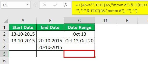
Now in case both the dates are missing, we could use a nested IF statement in Excel (i.e., one IF inside another IF statement) as follows:

Date Range =IF(A4<>””,TEXT(A4,”mmm d”) & IF(B4<> “”, “-” & TEXT(B4,”mmm d”), “”),””)

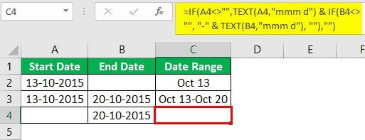
So we can see that the above formula returns an empty string if the start date is missing.

If both the dates are missing, an empty string is also returned.

• We can even create a list of sequential dates using the "Fill Handle" command. We can select the cell having a start date and then drag it to the range of cells where we wish to fill. Next, click on the "Home" tab - "Editing" -"Fill Series" and then choose a date unit we want to use.
• If we wish to calculate the duration or number of days between two dates, we can subtract the two dates using the '-'operator, and we will get the desired result.

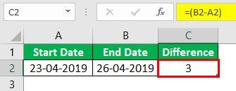
Note: The format of cells: A2 and B2 is ‘Date,’ whereas that of cell C2 is ‘General’ as it calculates the number of days.

This article has been a guide to Date Range in Excel. Here, we discuss formulas to create date ranges in Excel in different ways and a downloadable Excel template. You may learn more about Excel from the following articles: -

• DATE Excel Function
• EDATE Excel Function
• Subtract Date In Excel
• Compare Dates in Excel