
Table Of Contents
What is Hyperlink in Excel?
A hyperlink in excel takes the user to the intended location with a single click. This intended location can be a web page, worksheet, email address, file stored on a hard disk, and so on. A hyperlink is inserted in Excel to provide quick access to a related source of information.
For instance, while reviewing the financial statements in Excel, the auditor may be given access to the supporting documents of the organization. Such documents include invoices, receipts, purchase orders, etc., which may be attached to the worksheet through hyperlinks.
Once a hyperlink is created, its on-screen name is underlined and displayed in blue. This change of appearance is a proof that the hyperlink has become clickable. This article discusses the different techniques of inserting hyperlinks in Excel.
How to Insert a Hyperlink in Excel?
The methods of inserting a hyperlink in Excel are listed as follows:
- Default creation technique
- “Insert hyperlink” dialog box
- HYPERLINK function
Let us discuss each method one by one.
Method #1–Default Creation Technique
This is the easiest method of creating hyperlinks in Excel. It works when the intended location is a web page on the Internet.
Procedure to be Followed
The steps for inserting a hyperlink with the default method are listed as follows:
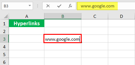
Step 1: Type the URL of the intended location in a cell. We have typed “www.google.com” in cell B3, as shown in the following image.
Note: A URL (uniform resource locator) is the address of a resource on the Internet. It is a unique web address that helps retrieve the resource.
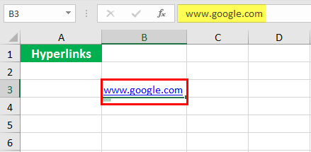
Step 2: Once the URL has been entered, press the “Enter” key. Excel automatically converts the URL to a clickable hyperlink. Notice that the URL in the following image is underlined and has turned blue.
Note: Ignore the green horizontal line displaying below the URL in the following image. This appears because cell B3 has been selected.
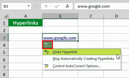
Undo the creation of a hyperlink: To undo the hyperlink created in the preceding step, follow the listed steps:
- Select the cell containing the hyperlink.
- Click the drop-down arrow of the AutoCorrect Options button. This button appears right below the cell containing the hyperlink.
- Click “undo hyperlink.”
In the succeeding image, the AutoCorrect Options button is shown in a red box and the “undo hyperlink” option is highlighted in green.
When a hyperlink is undone, the URL typed in Excel is considered simply as a text string.
Note 1: To select the cell containing the hyperlink (without being taken to the destination), use either of the following methods:
- Select an adjacent cell and use the arrow keys to select the cell containing the hyperlink.
- Click the cell containing the hyperlink and hold the mouse button until the cursor changes to a “cross” or “plus” sign. Once the cursor assumes this sign, release the mouse button.
Note 2: To stop Excel from creating automatic hyperlinks, select the option “stop automatically creating hyperlinks” from the AutoCorrect Options button.
Alternatively, from the AutoCorrect Options button, click “control AutoCorrect options.” The AutoCorrect dialog box will open. Switch to the tab “AutoFormat as you type.” Deselect the checkbox of “internet and network paths with hyperlinks.” This will prevent Excel from creating automatic hyperlinks.
Method #2–“Insert Hyperlink” Dialog Box
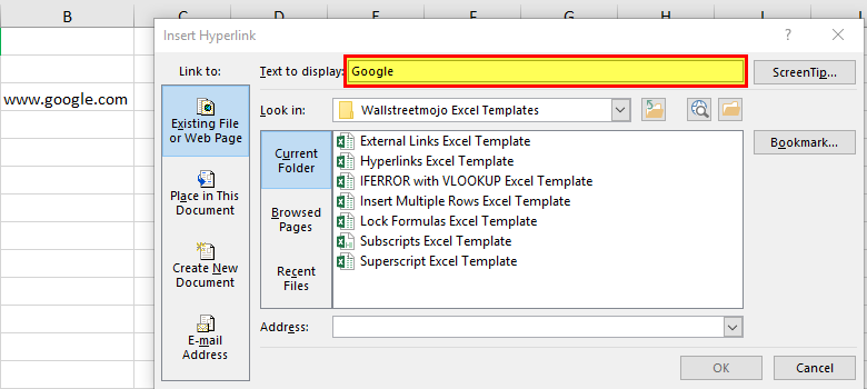
“Insert Hyperlink” is a dialog box that can be accessed from the Insert tab of Excel. This box helps create hyperlinks based on the kind of destination specified by the user.
This dialog box also allows creating a screen tip by clicking the “ScreenTip” option on the top-right side. A screen tip is a customized message displayed when the cursor rests on the hyperlink.
Procedure to be Followed
The steps to insert a hyperlink by using the “insert hyperlink” dialog box are listed as follows:
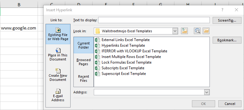
Step 1: Select the cell where a hyperlink needs to be inserted. We have selected the blank cell B3. Next, click “hyperlink” from the “links” group of the Insert tab. The “insert hyperlink” dialog box opens, as shown in the following image.
Alternatively, once the cell is selected, press the keys “Ctrl+K” together. For Excel for Mac, press the keys “Command+K.”
Note: Another approach is to right-click the selected cell and choose “hyperlink” from the context menu. This also opens the “insert hyperlink” dialog box.
Step 2: In “text to display,” type the on-screen name the way it should appear in the worksheet. We have typed “Google,” as shown in the following image.
Under “link to,” let the option “existing file or web page” remain selected. Likewise, under “look in,” let the option “current folder” remain selected.
Further, in the address box, type “www.google.com.” As the user types this path, Excel automatically inserts the web address as “http://www.google.com/.” This implies that “http,” colon (:), and forward slashes (/) are inserted at the right places by Excel.
Once the address has been entered, click “Ok.”
Note: The “Ok” button will become clickable as soon as the first letter is typed in the address box.
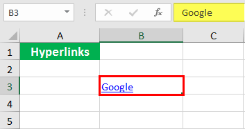
Step 3: Once “Ok” is clicked in the preceding step, a hyperlink with the on-screen name “Google” is created. This is shown in cell B3 of the following image.
Clicking the hyperlink “Google” takes the user to its website. Hence, a display text (on-screen name) and a web address are the two requirements for creating a hyperlink connected to a web page.
Method #3–HYPERLINK Function
A hyperlink can be inserted by using the HYPERLINK function of Excel. This method is particularly helpful when multiple hyperlinks need to be created at a time.
The syntax of the HYPERLINK function is shown in the following image:
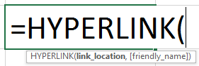
The HYPERLINK function accepts the following arguments:
- Link_location: This is the path to the intended location. It is supplied as a text string enclosed within double quotation marks or a reference to a cell containing the text string.
- Friendly_name: This is the on-screen name (or jump text) displayed in Excel. It is supplied as a text string enclosed within double quotation marks, numeric value or a reference to a cell containing the on-screen name.
The “link_location” argument is required, while “friendly_name” is optional. If the latter is omitted, the “link_location” is retained as the on-screen name.
Procedure to be Followed
The steps to insert a hyperlink by using the HYPERLINK function of Excel are listed as follows:
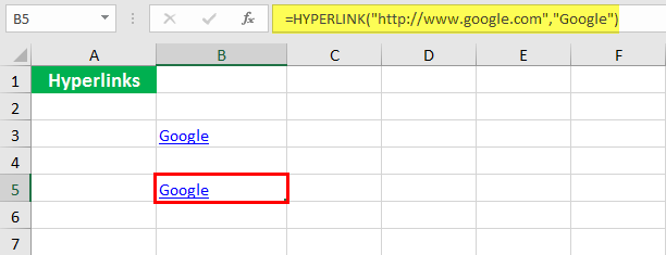
Step 1: Supply the “link_location” and the “friendly_name” to the HYPERLINK function. So, enter the following HYPERLINK formula (without the beginning and ending double quotation marks) in any cell, say B5.
“=HYPERLINK(“http://www.google.com”,“Google”)”
In this formula, the path of the intended location is “http://www.google.com” and the on-screen name is “Google.”
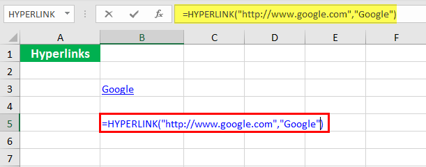
Step 2: Press the “Enter” key. A hyperlink named “Google” is created in cell B5. This is shown within a red box in the following image.
Examples
Let us consider a few examples of creating hyperlinks with the HYPERLINK function of Excel.
#1–Insert Multiple Hyperlinks with Web Pages as the Destination
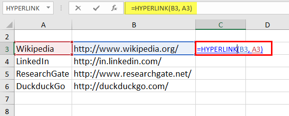
The following image shows a list of URLs in the range B3:B6. For each URL, the corresponding on-screen name is given in the range A3:A6. Create hyperlinks that link the given names to their respective URLs.
Use the HYPERLINK function of Excel.

The steps to create multiple hyperlinks by using the HYPERLINK function are listed as follows:
Step 1: Supply the cell references containing the “link_location” (or the URL) and the “friendly_name.” So, enter the following formula in cell C3.
“=HYPERLINK(B3,A3)”
Step 2: Press the “Enter” key. A hyperlink named “Wikipedia” is created in cell C3 of the following image.
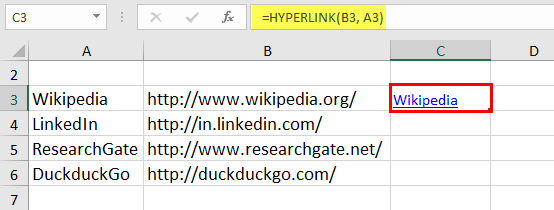
Step 3: Drag the formula of cell C3 till cell C6. For this, use the fill handle displayed at the bottom-right side of cell C3.
The dragging of the fill handle and the outputs are shown in the following image. Hence, clicking any of the created hyperlinks (in C3:C6) will take the user to the respective web page.
#2–Insert Multiple Hyperlinks with Pictures as the Destination
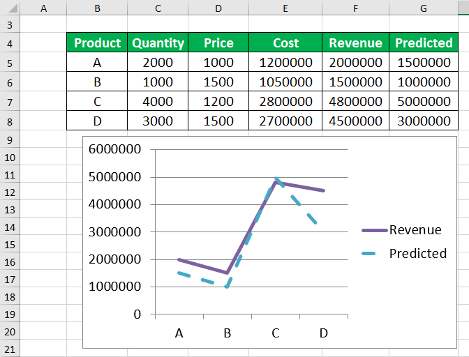
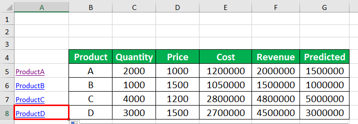
The following image shows the quantities sold (column C), prices (column D), costs (column E), predicted revenues (column G), and actual revenues (column F) for four products (A, B, C, and D) of an organization.
Further, the following information is shared:
- All figures of columns D, E, F, and G are in US dollars. The entire dataset pertains to a specific month of the year 2018.
- A line chart has been inserted (below the dataset) to illustrate the difference between the predicted and the actual revenues.
- Each product has been assigned a picture whose title matches the name of the product. So, the pictures are titled A.png, B.png, C.png, and D.png. All these pictures are stored in a folder whose location has been given (in cell J12) as: file://localhost/Users/parul/Desktop/Excel functions/Hyperlinks/
Create four hyperlinks titled “Product A,” “Product B,” “Product C,” and “Product D.” Place these hyperlinks to the left of the dataset. When clicked, each hyperlink should take the user to the corresponding picture of the product.
Use the HYPERLINK function of Excel.
The steps for creating hyperlinks with pictures as the destination are listed as follows:
Step 1: Enter the following HYPERLINK formula in cell A5.
“=HYPERLINK(($J$12&B5&".png"),"Product "&B5)”
This formula is shown in the following image.
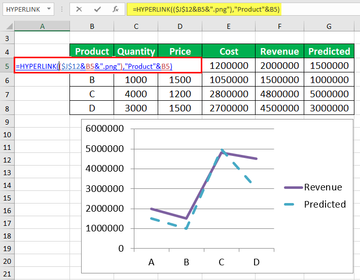
Explanation of the formula: In the preceding formula, the ampersand operator (&) is used to join the values of cells J12 (location of the pictures) and B5 (letter A) with the extension “.png.” The parentheses preceding the comma ($J$12&B5&".png") serve as the “link_location.” So, the entire “link_location” is:
file://localhost/Users/parul/Desktop/Excel functions/Hyperlinks/A.png
The argument succeeding the comma ("Product "&B5) serves as the “friendly_name.” In this argument, the word “product” is joined with the letter A (in cell B5) to form the on-screen name.
Notice that a single space has been inserted in the formula after the word “product.” This is because we want a space to separate the two strings of the on-screen name (like “Product A”). However, this space may not be visible in the formula of the preceding image.
In other words, the entire formula we entered in the preceding step is stated as follows:
“=HYPERLINK("file://localhost/Users/parul/Desktop/Excel functions/Hyperlinks/A.png","Product A")”
Had this formula been entered directly (without the beginning and ending double quotation marks), it would have worked the same way the present formula of step 1 works.
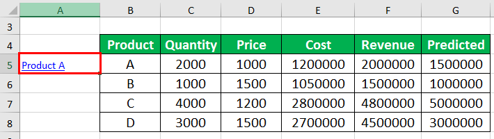
Step 2: Press the “Enter” key. A hyperlink named “Product A” is created in cell A5. This is shown in a red box in the following image.
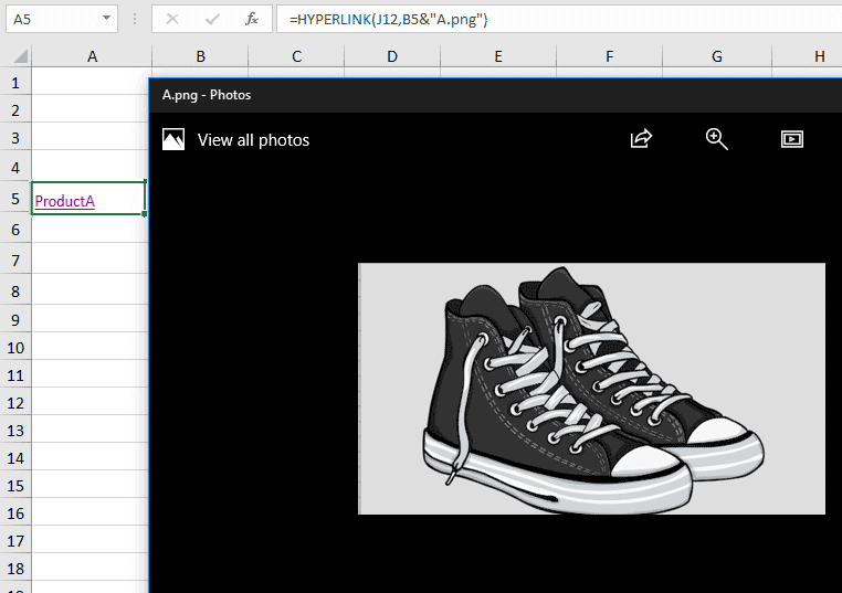
Step 3: Click the hyperlink created in the preceding step. The picture titled A.png opens. This picture had been assigned to product A.
The picture A.png is shown in the following image.
Step 4: Drag the formula of cell A5 till cell A8. The hyperlinks for all the products are created in this range. These are shown in the following image.
In this way, hyperlinks with pictures as the destination have been created in Excel.
Use of Inserting a Hyperlink in Excel
The common uses of inserting a hyperlink in Excel are listed as follows:
- It helps navigate to a file or web page on the Internet or intranet.
- It helps send emails from the default email account of the user.
- It helps jump to a specific area in the workbook.
- It aids in opening a new Excel workbook.
- It makes the objects of a worksheet clickable.
